Add points or lines to an L-moment ratio diagram

lmrdpoints adds points, and lmrdlines adds connected line segments, to an \(L\)-moment ratio diagram.

lmrdpoints(x, y=NULL, type="p", ...)
lmrdlines(x, y=NULL, type="l", ...)

Arguments

x

Numeric vector of \(L\)-skewness values.

y

Numeric vector of \(L\)-kurtosis values. May be omitted: see “Details” below.

type

Character indicating the type of plotting. Can be any valid value for the type argument of plot.default.

...

Further arguments (graphics parameters), passed to points or lines.

Details

The functions lmrdpoints and lmrdlines are equivalent to points and lines respectively, except that if argument y is omitted, x is assumed to be an object that contains both \(L\)-skewness and \(L\)-kurtosis values. As in lmrd, it can be a vector with elements named "t_3" and "t_4" (or "tau_3" and "tau_4"), a matrix or data frame with columns named "t_3" and "t_4" (or "tau_3" and "tau_4"), or an object of class "regdata" (as defined in package lmomRFA).

Author

J. R. M. Hosking jrmhosking@gmail.com

See also

lmrd, points, lines.

Examples

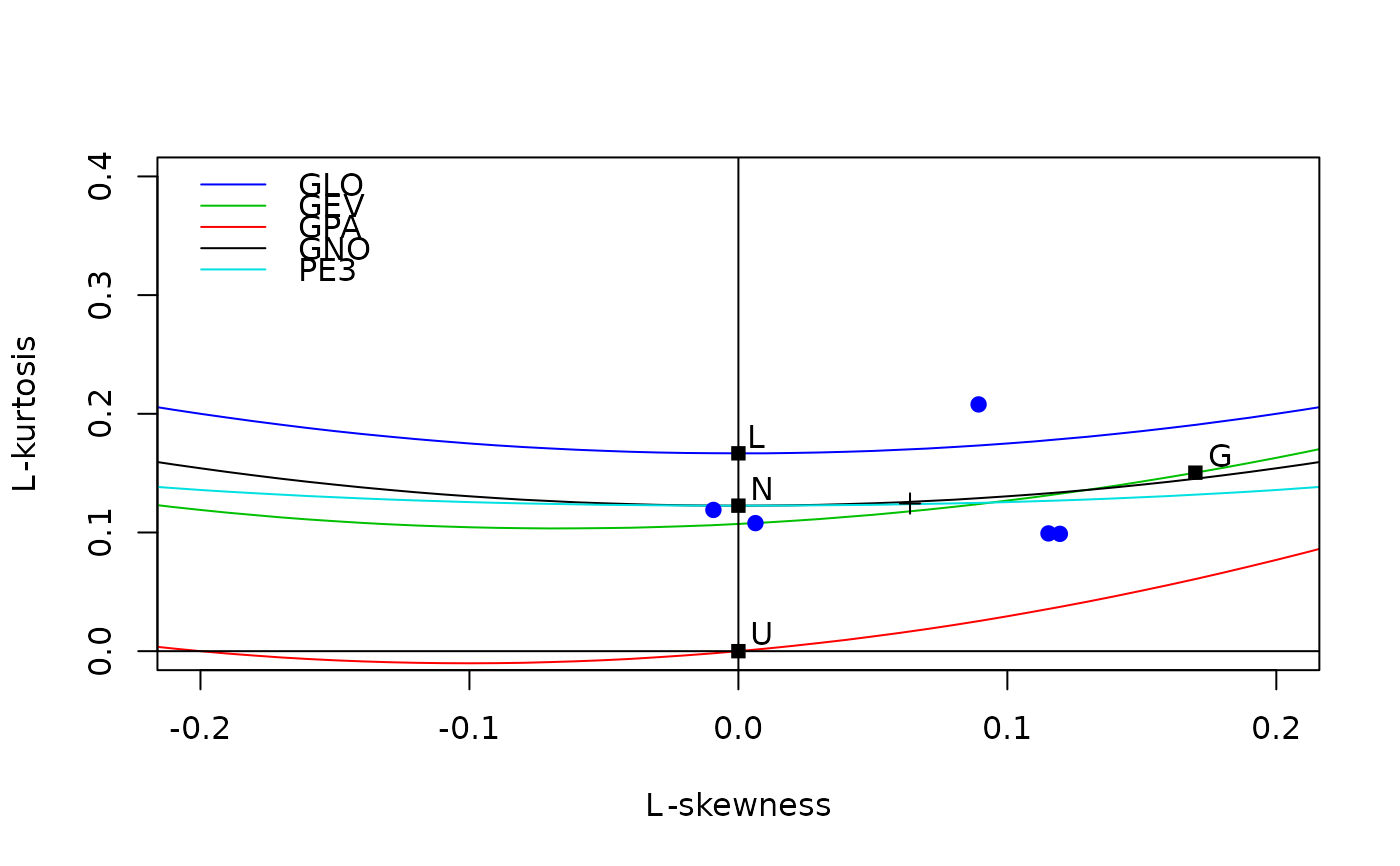
# Plot L-moment ratio diagram of Wind from the airquality data set
data(airquality)
lmrd(samlmu(airquality$Wind), xlim=c(-0.2, 0.2))
# Sample L-moments of each month's data
( lmom.monthly <- with(airquality,
  t(sapply(5:9, function(mo) samlmu(Wind[Month==mo])))) )
#>            l_1      l_2          t_3        t_4
#> [1,] 11.622581 2.021935  0.115287283 0.09921692
#> [2,] 10.266667 2.086437  0.089301454 0.20791010
#> [3,]  8.941935 1.738065  0.119524870 0.09885496
#> [4,]  8.793548 1.859570  0.006328685 0.10788844
#> [5,] 10.180000 1.993793 -0.009289915 0.11901376
# Add the monthly values to the plot
lmrdpoints(lmom.monthly, pch=19, col="blue")



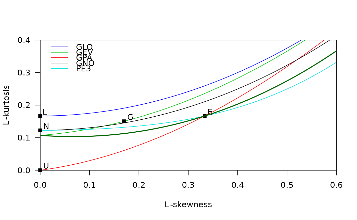
# Draw an L-moment ratio diagram and add a line for the
# Weibull distribution
lmrd(xaxs="i", yaxs="i", las=1)
weimom <- sapply( seq(0, 0.9, by=0.01),
  function(tau3) lmrwei(pelwei(c(0,1,tau3)), nmom=4) )
lmrdlines(t(weimom), col='darkgreen', lwd=2)