L-moment ratio diagram

Draws an \(L\)-moment ratio diagram.

lmrd(x, y, distributions = "GLO GEV GPA GNO PE3", twopar,
     xlim, ylim, pch=3, cex, col, lty, lwd=1,
     legend.lmrd = TRUE, xlegend, ylegend,
     xlab = expression(italic(L) * "-skewness"),
     ylab = expression(italic(L) * "-kurtosis"), ...)

Arguments

x

Numeric vector of \(L\)-skewness values.

Alternatively, if argument y is omitted, x can be an object that contains both \(L\)-skewness and \(L\)-kurtosis values. It can be a vector with elements named "t_3" and "t_4" (or "tau_3" and "tau_4"), a matrix or data frame with columns named "t_3" and "t_4" (or "tau_3" and "tau_4"), or an object of class "regdata" (as defined in package lmomRFA).

y

Numeric vector of \(L\)-kurtosis values.

distributions

Indicates the three-parameter distributions whose \(L\)-skewness–\(L\)-kurtosis relations are to be plotted as lines on the diagram. The following distribution identifiers are recognized, in upper or lower case:

	`GLO`	generalized logistic
	`GEV`	generalized extreme-value
	`GPA`	generalized Pareto
	`GNO`	generalized normal
	`PE3`	Pearson type III
	`WAK.LB`	lower bound of \(L\)-kurtosis for given \(L\)-skewness,
		for the Wakeby distribution.
	`ALL.LB`	lower bound of \(L\)-kurtosis for given \(L\)-skewness,
		for all distributions.

The argument should be either a character vector each of whose elements is one of the above abbreviations or a character string containing one or more of the abbreviations separated by blanks. The specified \(L\)-skewness–\(L\)-kurtosis curves will be plotted.

If no three-parameter distributions are to be plotted, specify distributions to be FALSE or the empty string, "".

twopar

Two-parameter distributions whose (\(L\)-skewness, \(L\)-kurtosis) values are to be plotted as points on the diagram. The following distribution identifiers are recognized, in upper or lower case:

	`E` or `EXP`	exponential
	`G` or `GUM`	Gumbel
	`L` or `LOG`	logistic
	`N` or `NOR`	normal
	`U` or `UNI`	uniform

The argument should be either a character vector each of whose elements is one of the above abbreviations or a character string containing one or more of the abbreviations separated by blanks. \(L\)-skewness–\(L\)-kurtosis points for the specified distributions will be plotted and given one-character labels.

The default is to plot the two-parameter distributions that are special cases of the three-parameter distributions specified in argument distributions. Thus for example if distributions="GPA PE3", the default for twopar is "EXP NOR UNI": NOR is a special case of PE3, UNI of GPA, EXP of both GPA and PE3.

If no two-parameter distributions are to be plotted, specify twopar to be FALSE or the empty string, "".

xlim

x axis limits. Default: c(0, 0.6), expanded if necessary to cover the range of the data.

ylim

y axis limits. Default: c(0, 0.4), expanded if necessary to cover the range of the data.

pch

Plotting character to be used for the plotted (\(L\)-skewness, \(L\)-kurtosis) points.

cex

Symbol size for plotted points, like graphics parameter cex.

col

Vector specifying the colors. If it is of length 1 and x is present, it will be used for the plotted points. Otherwise it will be used for the lines on the plot. For the default colors for the lines, see the description of argument lty below.

lty

Vector specifying the line types to be used for the lines on the plot.

By default, colors and line types are matched to the distributions given in argument distributions, as follows:

	`GLO`	blue, solid line
	`GEV`	green, solid line
	`GPA`	red, solid line
	`GNO`	black, solid line
	`PE3`	cyan, solid line
	`WAK.LB`	red, dashed line
	`ALL.LB`	black, dashed line

The green and cyan colors are less bright than the standard "green" and "cyan"; they are defined to be "#00C000" and "#00E0E0", respectively.

lwd

Vector specifying the line widths to be used for the lines on the plot.

legend.lmrd

Controls whether a legend, identifying the \(L\)-skewness–\(L\)-kurtosis relations of the three-parameter distributions, is plotted. Either logical, indicating whether a legend is to be drawn, or a list specifying arguments to the legend function. Default arguments include bty="n", which must be overridden if a legend box is to be drawn; other arguments set by default are x, y, legend, col, lty, and lwd.

Not used if distributions is FALSE.

xlegend, ylegend

x and y coordinates of the upper left corner of the legend. Default: coordinates of the upper left corner of the plot region, shifted to the right and downwards, each by an amount equal to 1% of the range of the x axis.

Not used if distributions is FALSE or if legend.lmrd is FALSE.

xlab

X axis label.

ylab

Y axis label.

...

Additional arguments are passed to the function matplot, which draws the axis box and the lines for three-parameter distributions.

Details

lmrd calls a sequence of graphics functions: matplot for the axis box and the curves for three-parameter distributions; points for the points for two-parameter distributions and text for their labels; legend for the legend; and points for the \((x,y)\) data points.

Note that the only graphics parameters passed to points are col (if of length 1), cex, and pch. If more complex features are required, such as different colors for different points, follow lmrd by an additional call to points, e.g. follow lmrd(t3, t4) by points(t3, t4, col=c("red", "green")).

Value

A list, returned invisibly, describing what was plotted. Useful for customization of the legend, as in one of the examples below. List elements:

lines: List containing elements describing the plotted distribution curves (if any). Each element is a vector with the same length as distributions. List elements distributions, col.lines, lty, lwd.
twopar: Character vector containing the 1-character symbols for the two-parameter distributions that were plotted.
points: List containing elements describing the plot (if any) of the data points. List elements col.pts, pch, cex.

If any of the above items was not plotted, the corresponding list element is NULL.

Author

J. R. M. Hosking jrmhosking@gmail.com

Examples

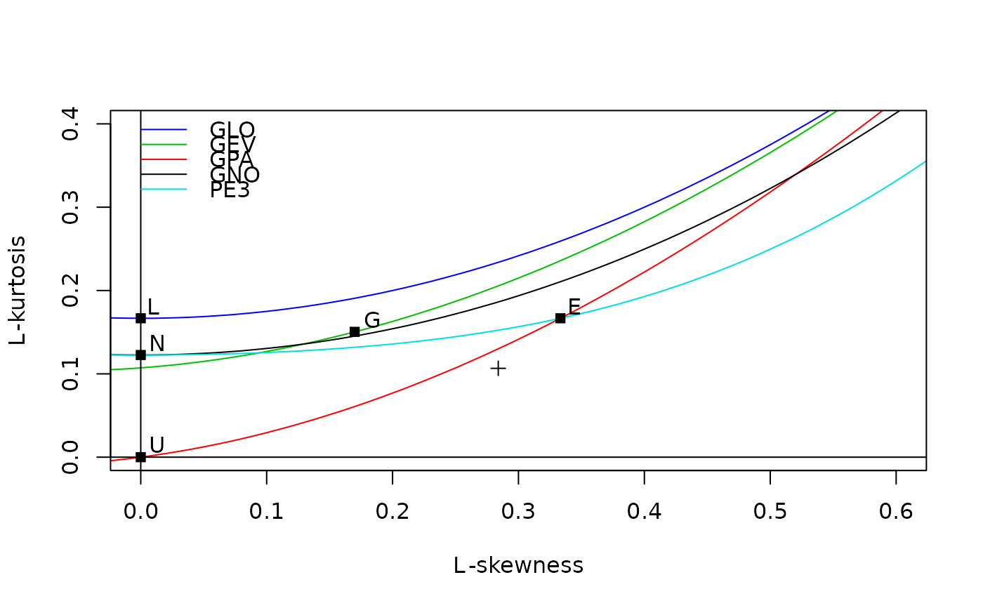
data(airquality)
lmrd(samlmu(airquality$Ozone))


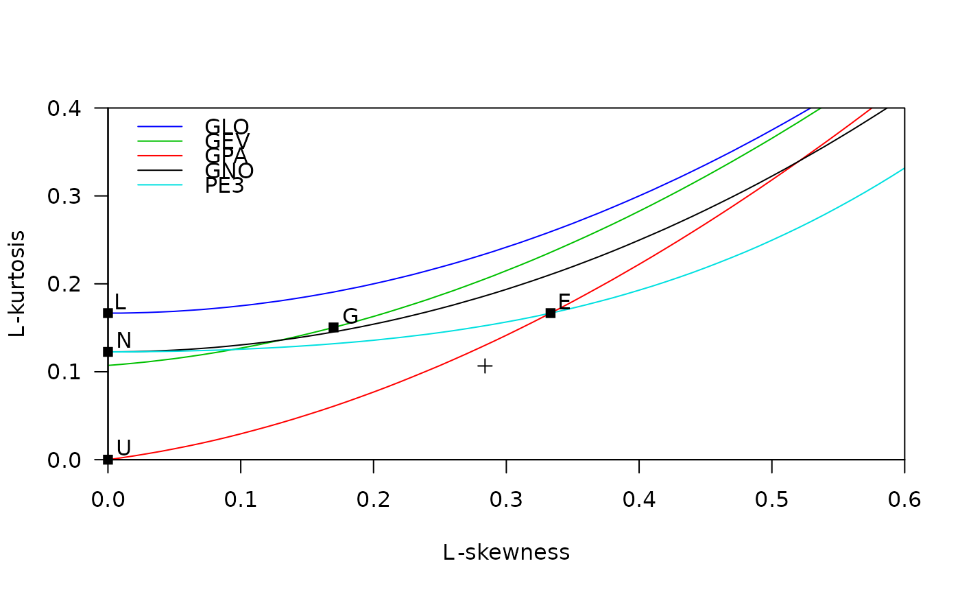
# Tweaking a few graphics parameters makes the graph look better
# (in the author's opinion)
lmrd(samlmu(airquality$Ozone), xaxs="i", yaxs="i", las=1)


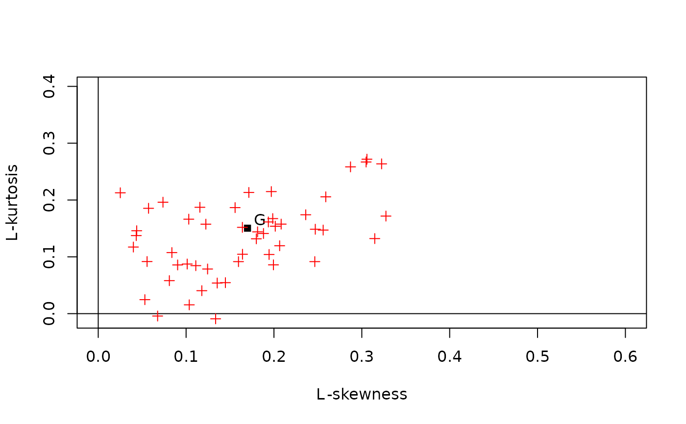
# An example that illustrates the sampling variability of L-moments
#
# Generate 50 random samples of size 30 from the Gumbel distribution
# - stored in the rows of matrix mm
mm <- matrix(quagum(runif(1500)), nrow=50)
#
# Compute the first four sample L-moments of each sample
# - stored in the rows of matrix aa
aa <- apply(mm, 1, samlmu)
#
# Plot the L-skewness and L-kurtosis values on an L-moment ratio
# diagram that also shows (only) the population L-moment ratios
# of the Gumbel distribution
lmrd(t(aa), dist="", twopar="G", col="red")


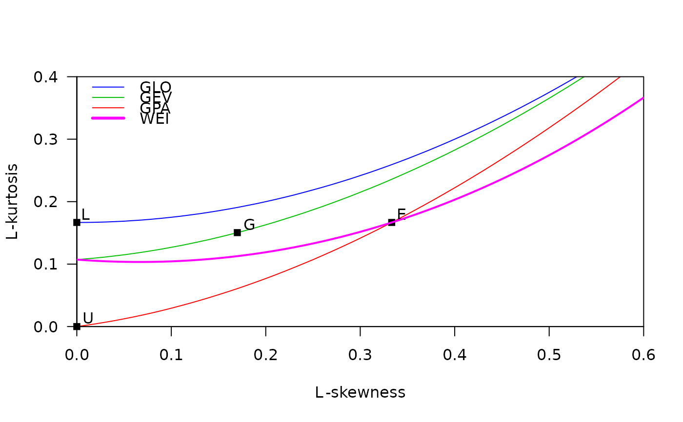
# L-moment ratio diagram with curves for GLO, GEV, GPA, and Weibull.
# The Weibull curve is added manually. A legend is added,
# using information returned from lmrd().
#
# - Draw the diagram, with the GLO, GEV, and GPA curves
info <- lmrd(distributions="GLO GEV GPA", xaxs="i", yaxs="i", las=1, legend=FALSE)
#
# - Compute L-skewness and L-kurtosis values for Weibull
sa <- sapply(seq(0, 0.6, by=0.01),
    function(tau3) lmrwei(pelwei(c(0,1,tau3)), nmom=4)[3:4])
#
# - Plot the Weibull curve
lmrdlines(sa["tau_3",], sa["tau_4",], col="magenta", lwd=2)
#
# - Add a legend
legend("topleft", bty="n",
  legend = c(info$lines$distributions, "WEI"),
  col = c(info$lines$col.lines, "magenta"),
  lwd = c(info$lines$lwd, 3))

Arguments

Details

Value

Author

See also

Examples