stat_peaks finds at which x positions the global y maximun or local
y maxima are located. stat_valleys finds at which x positions the
global y minimum or local y minima located. They both support filtering
of relevant peaks. Axis flipping is supported.
stat_peaks(
  mapping = NULL,
  data = NULL,
  geom = "point",
  position = "identity",
  ...,
  span = 5,
  global.threshold = 0,
  local.threshold = 0,
  local.reference = "median",
  strict = FALSE,
  label.fmt = NULL,
  x.label.fmt = NULL,
  y.label.fmt = NULL,
  extract.peaks = NULL,
  orientation = "x",
  na.rm = FALSE,
  show.legend = FALSE,
  inherit.aes = TRUE
)

stat_valleys(
  mapping = NULL,
  data = NULL,
  geom = "point",
  position = "identity",
  ...,
  span = 5,
  global.threshold = 0.01,
  local.threshold = NULL,
  local.reference = "median",
  strict = FALSE,
  label.fmt = NULL,
  x.label.fmt = NULL,
  y.label.fmt = NULL,
  extract.valleys = NULL,
  orientation = "x",
  na.rm = FALSE,
  show.legend = FALSE,
  inherit.aes = TRUE
)
Arguments
- mapping
The aesthetic mapping, usually constructed with
aesoraes_. Only needs to be set at the layer level if you are overriding the plot defaults.- data
A layer specific dataset - only needed if you want to override the plot defaults.
- geom
The geometric object to use display the data
- position
The position adjustment to use for overlapping points on this layer
- ...
other arguments passed on to
layer. This can include aesthetics whose values you want to set, not map. Seelayerfor more details.- span
odd positive integer A peak is defined as an element in a sequence which is greater than all other elements within a moving window of width
spancentred at that element. The default value is 5, meaning that a peak is taller than its four nearest neighbours.span = NULLextends the span to the whole length ofx.- global.threshold
numeric A value belonging to class
"AsIs"is interpreted as an absolute minimum height or depth expressed in data units. A barenumericvalue (normally between 0.0 and 1.0), is interpreted as relative to the range of the data. In both cases it sets a global height (depth) threshold below which peaks (valleys) are ignored. A bare negativenumericvalue indicates the global height (depth) threshold below which peaks (valleys) are be ignored. Ifglobal.threshold = NULL, no threshold is applied and all peaks are returned.- local.threshold
numeric A value belonging to class
"AsIs"is interpreted as an absolute minimum height (depth) expressed in data units relative to the within-window computed minimum (maximum) value. A barenumericvalue (normally between 0.0 and 1.0), is interpreted as expressed in units relative to the range of the data. In both caseslocal.thresholdsets a local height (depth) threshold below which peaks (valleys) are ignored. Iflocal.threshold = NULLor ifspanspans the whole ofx, no threshold is applied.- local.reference
character One of
"minimum"/maximumor"median". The reference used to assess the height of the peak, either the minimum value within the window or the median of all values in the window.- strict
logical flag: if
TRUE, an element must be strictly greater than all other values in its window to be considered a peak.- label.fmt, x.label.fmt, y.label.fmt
character strings giving a format definition for construction of character strings labels with function
sprintffromxand/oryvalues.- extract.peaks, extract.valleys
If
TRUEonly the rows containing peaks or valleys are returned. IfFALSEthe whole ofdatais returned but with labels set toNAin rows not containing peaks or valleys. IfNULL, the default,TRUE, is used unless the geom name passed as argument is"text_repel"or"label_repel".- orientation
character The orientation of the layer can be set to either
"x", the default, or"y".- na.rm
a logical value indicating whether NA values should be stripped before the computation proceeds.
- show.legend
logical. Should this layer be included in the legends?
NA, the default, includes if any aesthetics are mapped.FALSEnever includes, andTRUEalways includes.- inherit.aes
If
FALSE, overrides the default aesthetics, rather than combining with them. This is most useful for helper functions that define both data and aesthetics and shouldn't inherit behaviour from the default plot specification, e.g.borders.
Value
A data frame with one row for each peak (or valley) found in the
data extracted from the input data or all rows in data. Added
columns contain the labels.
Details
These stats use geom_point by default as it is the geom most
likely to work well in almost any situation without need of tweaking. The
default aesthetics set by these stats allow their direct use with
geom_text, geom_label, geom_line, geom_rug,
geom_hline and geom_vline. The formatting of the labels
returned can be controlled by the user.
Two tests make it possible to ignore irrelevant peaks or valleys. One test
controlled by (global.threshold) is based on the absolute
height/depth of peaks/valleys and can be used in all cases to ignore
globally low peaks and shallow valleys. A second test controlled by
(local.threshold) is available when the window defined by `span`
does not include all observations and can be used to ignore peaks/valleys
that are not locally prominent. In this second approach the height/depth of
each peak/valley is compared to a summary computed from other values within
the window where it was found. In this second case, the reference value
used is the summary indicated by local.reference. The values
global.threshold and local.threshold if bare numeric are
relative to the range of y. Thresholds for ignoring too small peaks
are applied after peaks are searched for, and threshold values can in some
cases result in no peaks being displayed.
Date time scales are recognized and labels formatted accordingly.
Note
These stats work nicely together with geoms geom_text_repel and
geom_label_repel from package ggrepel to
solve the problem of overlapping labels
by displacing them. To discard overlapping labels use check_overlap =
TRUE as argument to geom_text.
By default the labels are character values ready to be added as is, but
with a suitable label.fmt labels suitable for parsing by the geoms
(e.g. into expressions containing Greek letters or super or subscripts) can
be also easily obtained.
Computed and copied variables in the returned data frame
- x
x-value at the peak (or valley) as numeric
- y
y-value at the peak (or valley) as numeric
- x.label
x-value at the peak (or valley) formatted as character
- y.label
y-value at the peak (or valley) formatted as character
Default aesthetics
Set by the statistic and available to geoms.
- label
stat(x.label)
- xintercept
stat(x)
- yintercept
stat(y)
Required aesthetics
Required by the statistic and need to be set with aes().
- x
numeric, wavelength in nanometres
- y
numeric, a spectral quantity
See also
find_peaks, which is used internally.
find_peaks, for the functions used to located the
peaks and valleys.
Examples
# lynx and Nile are time.series objects recognized by
# ggpp::ggplot.ts() and converted on-the-fly with a default mapping
# numeric, date times and dates are supported with data frames
# using defaults
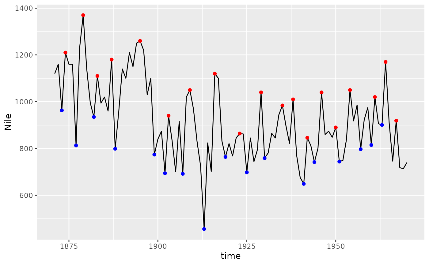
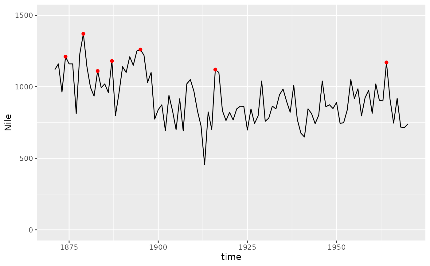
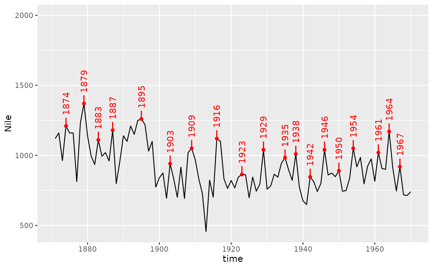
ggplot(Nile) +
geom_line() +
stat_peaks(colour = "red") +
stat_valleys(colour = "blue")
 # using wider window
ggplot(Nile) +
geom_line() +
stat_peaks(colour = "red", span = 11) +
stat_valleys(colour = "blue", span = 11)
# using wider window
ggplot(Nile) +
geom_line() +
stat_peaks(colour = "red", span = 11) +
stat_valleys(colour = "blue", span = 11)
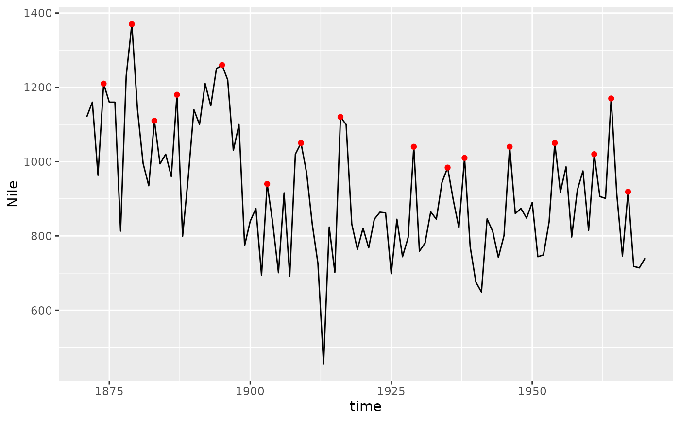
 # global threshold for peak height
ggplot(Nile) +
geom_line() +
stat_peaks(colour = "red",
global.threshold = 0.5) # half of data range
# global threshold for peak height
ggplot(Nile) +
geom_line() +
stat_peaks(colour = "red",
global.threshold = 0.5) # half of data range
 ggplot(Nile) +
geom_line() +
stat_peaks(colour = "red",
global.threshold = I(1100)) + # data unit
expand_limits(y = c(0, 1500))
ggplot(Nile) +
geom_line() +
stat_peaks(colour = "red",
global.threshold = I(1100)) + # data unit
expand_limits(y = c(0, 1500))
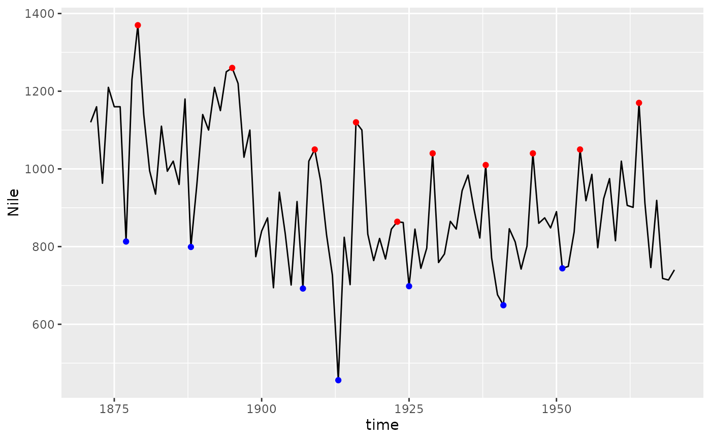
 # local (within window) threshold for peak height
# narrow peaks at the tip and locally tall
ggplot(Nile) +
geom_line() +
stat_peaks(colour = "red",
span = 9,
local.threshold = 0.3,
local.reference = "farthest")
# local (within window) threshold for peak height
# narrow peaks at the tip and locally tall
ggplot(Nile) +
geom_line() +
stat_peaks(colour = "red",
span = 9,
local.threshold = 0.3,
local.reference = "farthest")
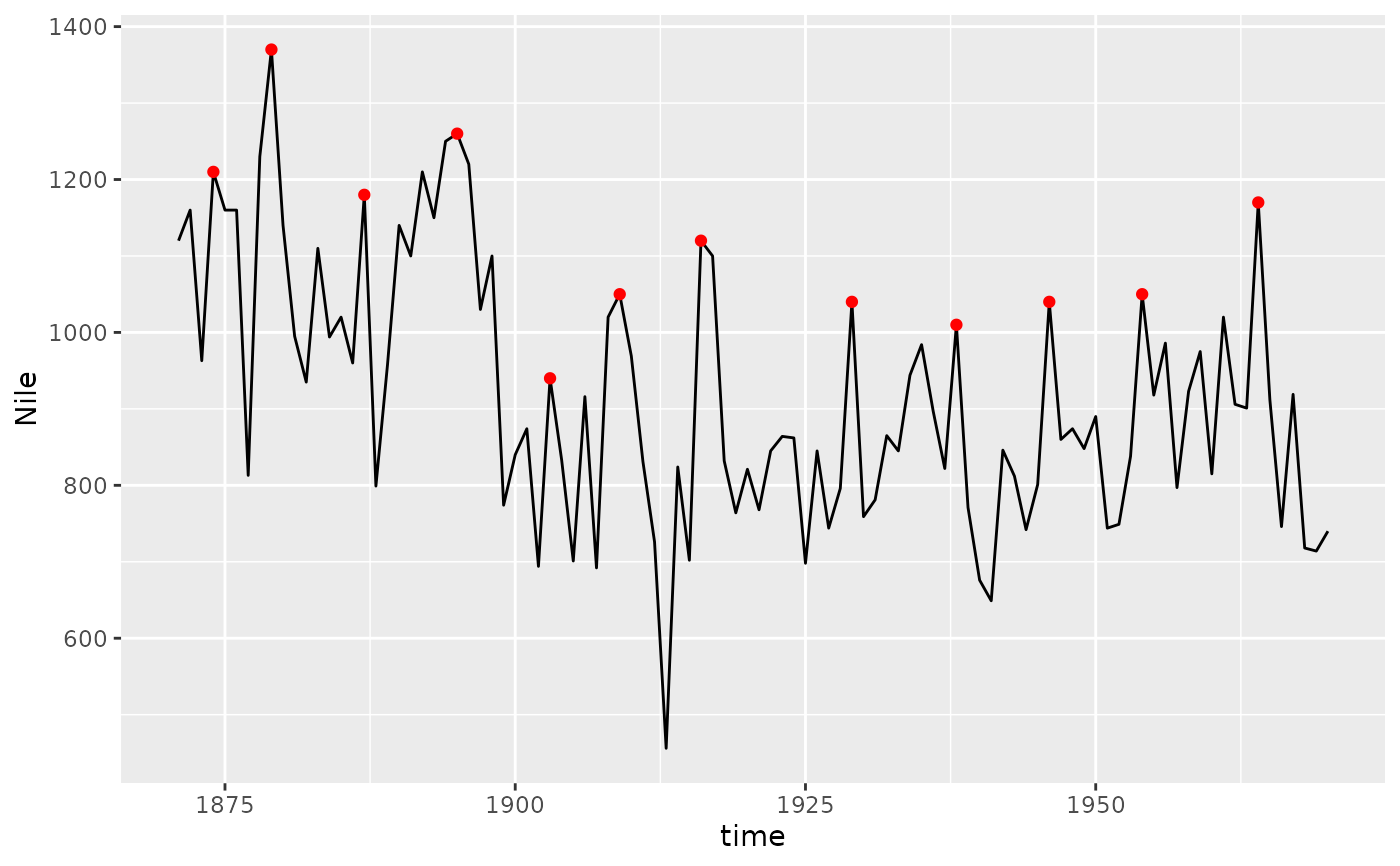
 # with narrower window
ggplot(Nile) +
geom_line() +
stat_peaks(colour = "red",
span = 5,
local.threshold = 0.25,
local.reference = "farthest")
# with narrower window
ggplot(Nile) +
geom_line() +
stat_peaks(colour = "red",
span = 5,
local.threshold = 0.25,
local.reference = "farthest")
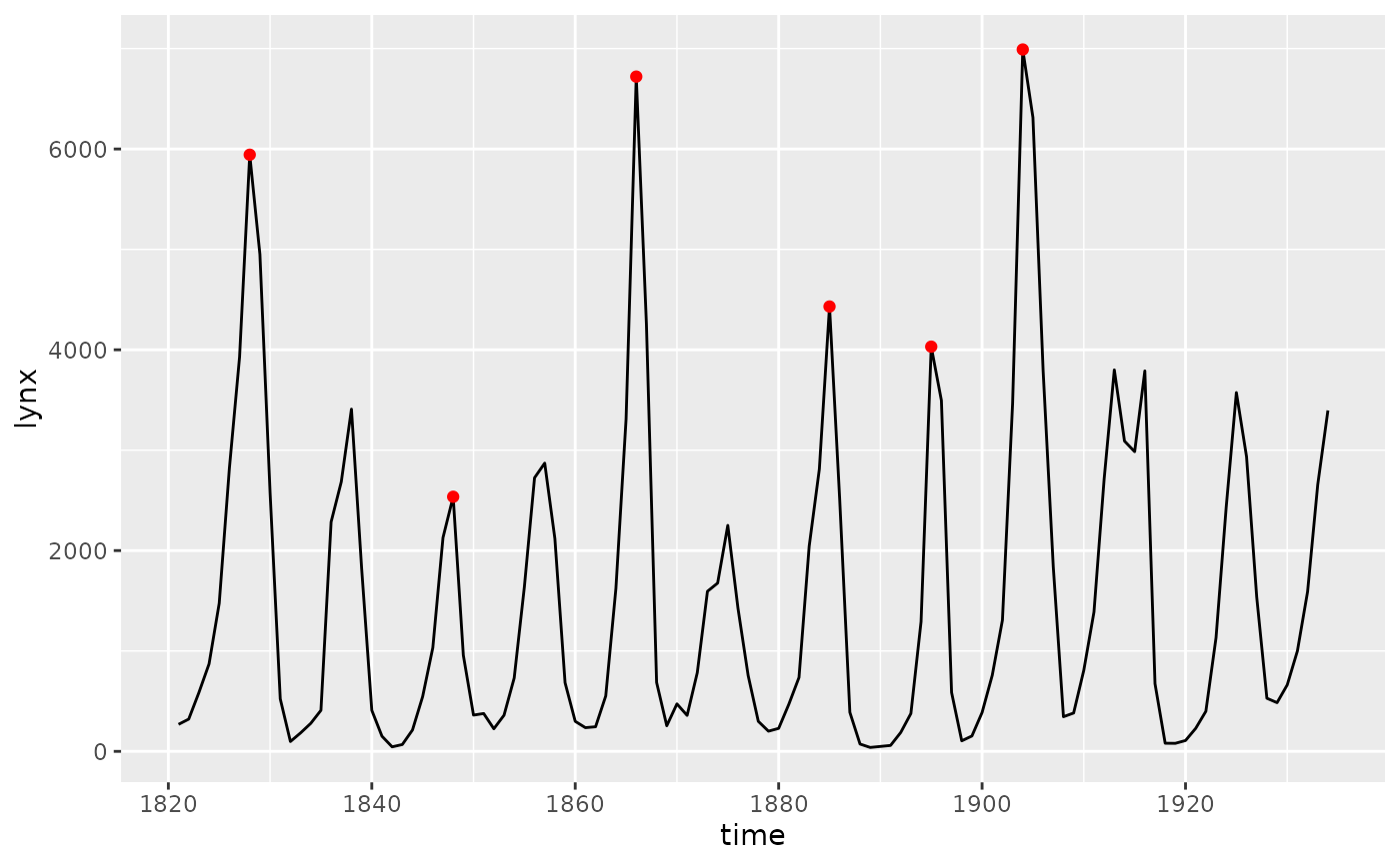
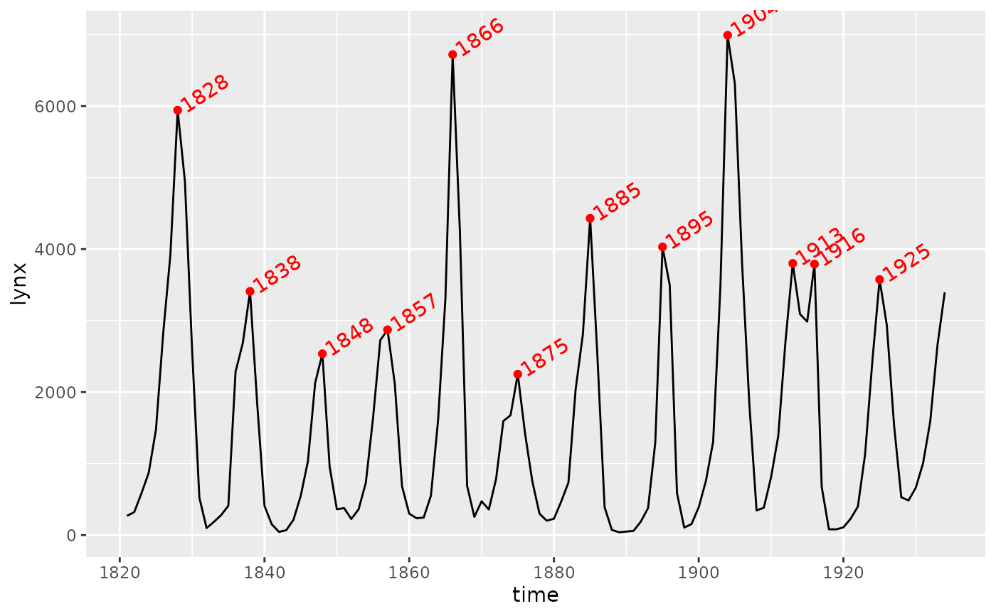
 ggplot(lynx) +
geom_line() +
stat_peaks(colour = "red",
local.threshold = 1/5,
local.reference = "median")
ggplot(lynx) +
geom_line() +
stat_peaks(colour = "red",
local.threshold = 1/5,
local.reference = "median")
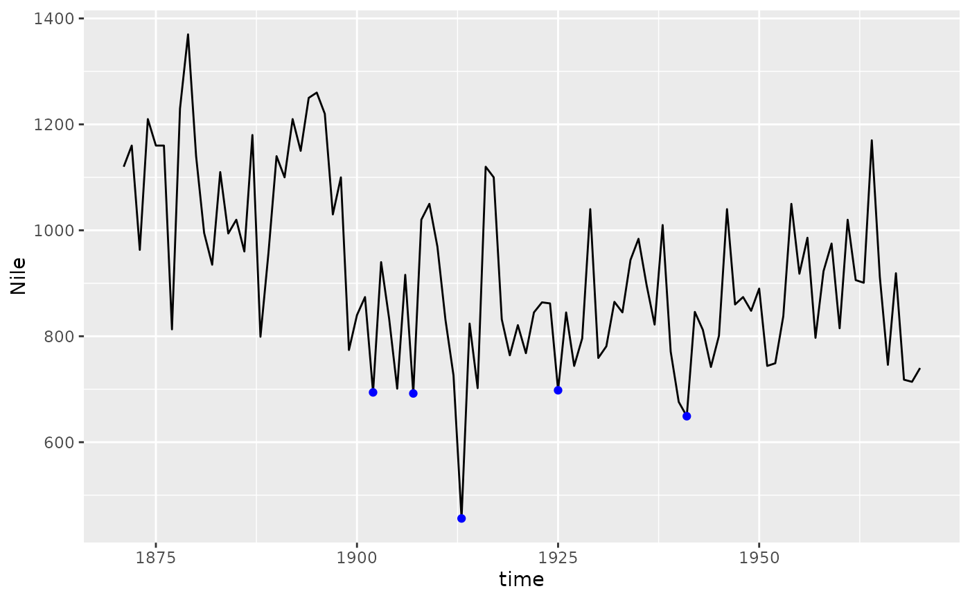
 ggplot(Nile) +
geom_line() +
stat_valleys(colour = "blue",
global.threshold = I(700))
ggplot(Nile) +
geom_line() +
stat_valleys(colour = "blue",
global.threshold = I(700))
 # orientation is supported
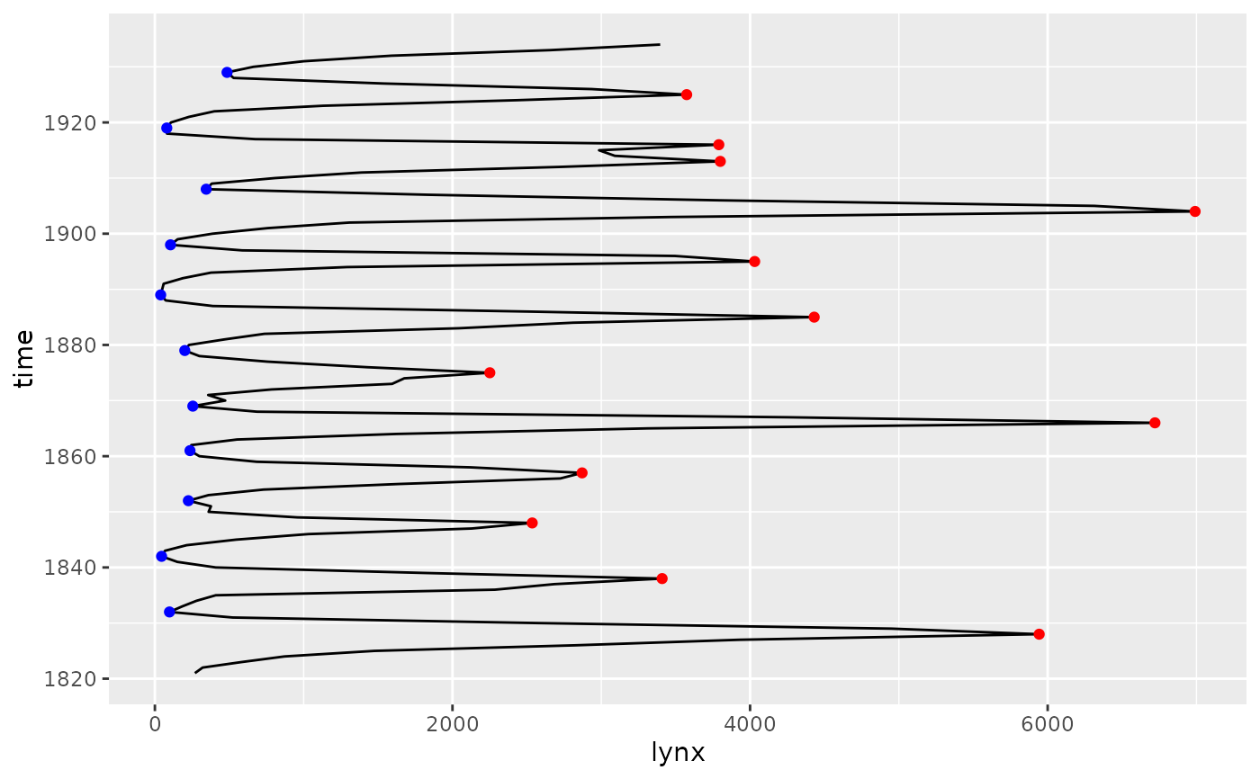
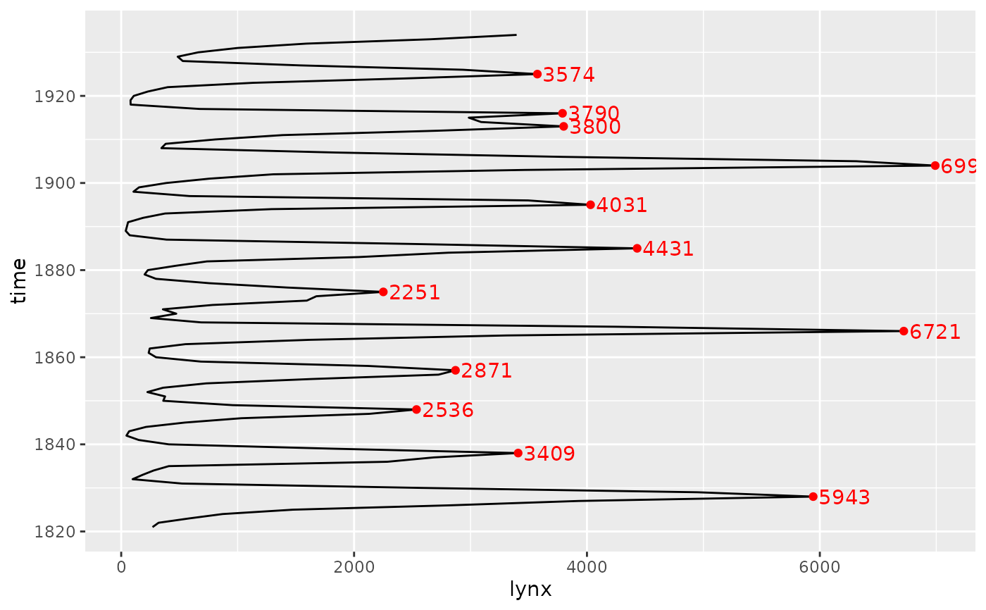
ggplot(lynx, aes(lynx, time)) +
geom_line(orientation = "y") +
stat_peaks(colour = "red", orientation = "y") +
stat_valleys(colour = "blue", orientation = "y")
# orientation is supported
ggplot(lynx, aes(lynx, time)) +
geom_line(orientation = "y") +
stat_peaks(colour = "red", orientation = "y") +
stat_valleys(colour = "blue", orientation = "y")
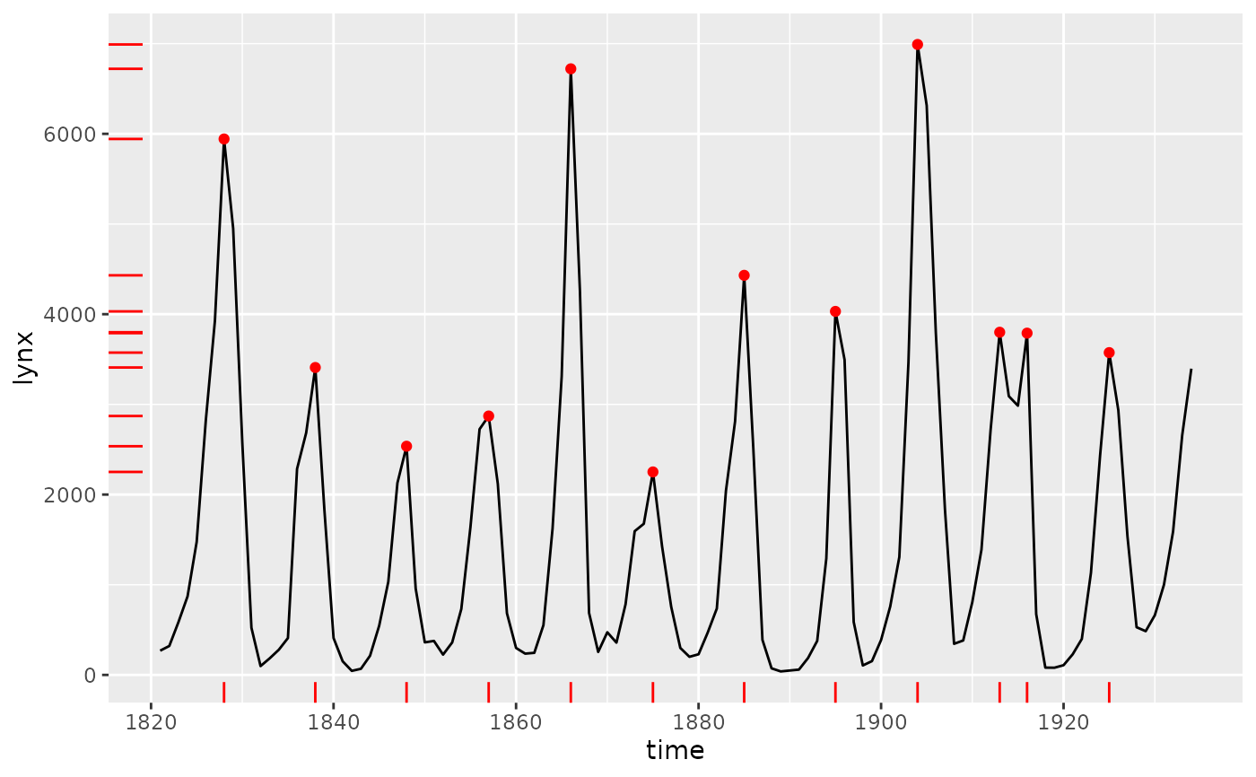
 # default aesthetic mapping supports additional geoms
ggplot(lynx) +
geom_line() +
stat_peaks(colour = "red") +
stat_peaks(colour = "red", geom = "rug")
# default aesthetic mapping supports additional geoms
ggplot(lynx) +
geom_line() +
stat_peaks(colour = "red") +
stat_peaks(colour = "red", geom = "rug")
 ggplot(lynx) +
geom_line() +
stat_peaks(colour = "red") +
stat_peaks(colour = "red", geom = "text", hjust = -0.1, angle = 33)
ggplot(lynx) +
geom_line() +
stat_peaks(colour = "red") +
stat_peaks(colour = "red", geom = "text", hjust = -0.1, angle = 33)
 ggplot(lynx, aes(lynx, time)) +
geom_line(orientation = "y") +
stat_peaks(colour = "red", orientation = "y") +
stat_peaks(colour = "red", orientation = "y",
geom = "text", hjust = -0.1)
ggplot(lynx, aes(lynx, time)) +
geom_line(orientation = "y") +
stat_peaks(colour = "red", orientation = "y") +
stat_peaks(colour = "red", orientation = "y",
geom = "text", hjust = -0.1)
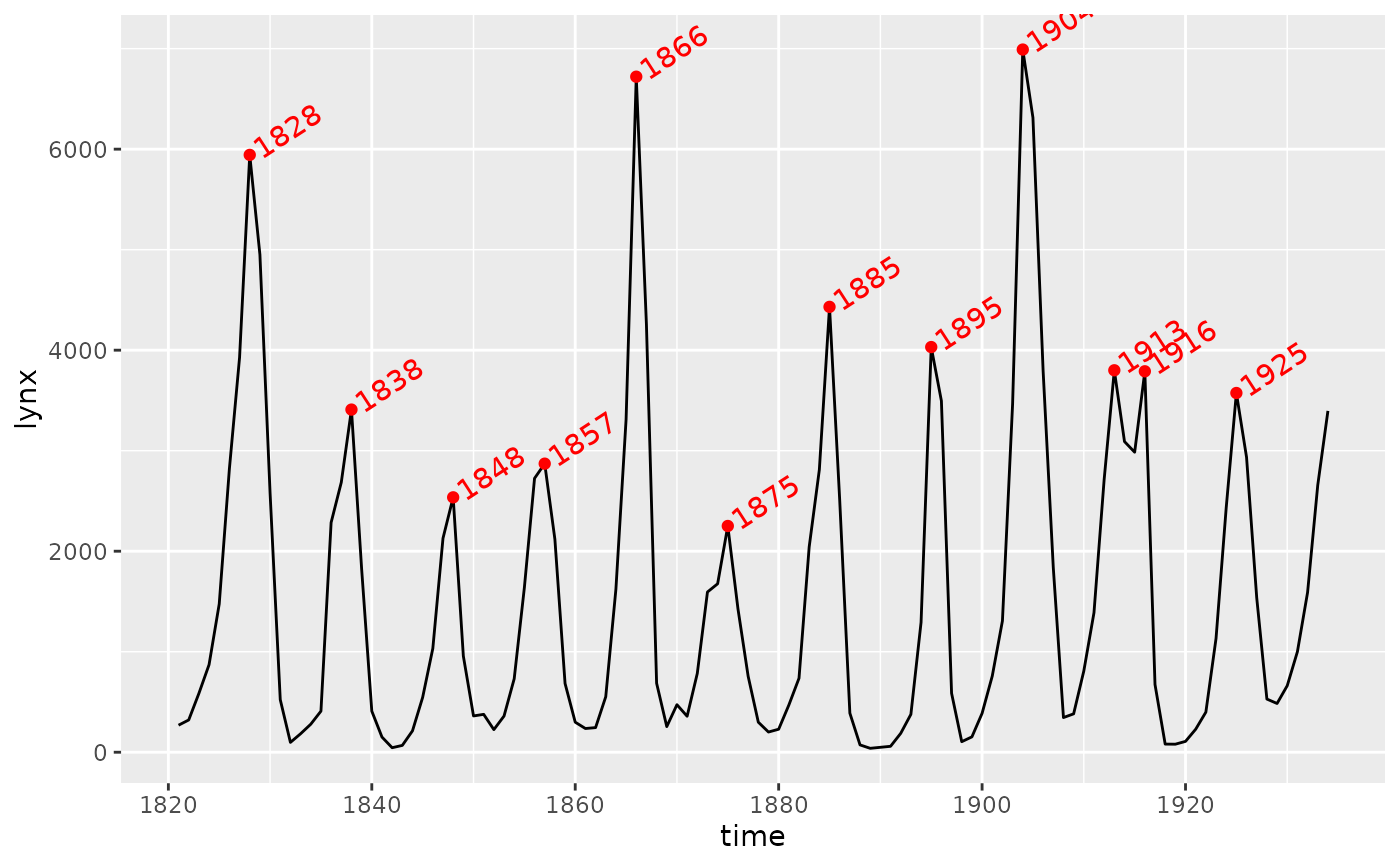
 # Force conversion of time series time into POSIXct date time
ggplot(lynx, as.numeric = FALSE) +
geom_line() +
stat_peaks(colour = "red") +
stat_peaks(colour = "red",
geom = "text",
hjust = -0.1,
x.label.fmt = "%Y",
angle = 33)
# Force conversion of time series time into POSIXct date time
ggplot(lynx, as.numeric = FALSE) +
geom_line() +
stat_peaks(colour = "red") +
stat_peaks(colour = "red",
geom = "text",
hjust = -0.1,
x.label.fmt = "%Y",
angle = 33)
 ggplot(Nile, as.numeric = FALSE) +
geom_line() +
stat_peaks(colour = "red") +
stat_peaks(colour = "red",
geom = "text_s",
position = position_nudge_keep(x = 0, y = 60),
hjust = -0.1,
x.label.fmt = "%Y",
angle = 90) +
expand_limits(y = 2000)
ggplot(Nile, as.numeric = FALSE) +
geom_line() +
stat_peaks(colour = "red") +
stat_peaks(colour = "red",
geom = "text_s",
position = position_nudge_keep(x = 0, y = 60),
hjust = -0.1,
x.label.fmt = "%Y",
angle = 90) +
expand_limits(y = 2000)
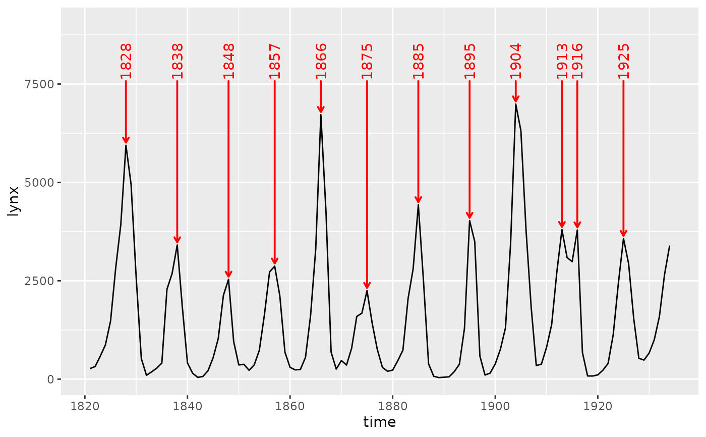
 ggplot(lynx, as.numeric = FALSE) +
geom_line() +
stat_peaks(colour = "red",
geom = "text_s",
position = position_nudge_to(y = 7600),
arrow = arrow(length = grid::unit(1.5, "mm")),
point.padding = 0.7,
x.label.fmt = "%Y",
angle = 90) +
expand_limits(y = 9000)
ggplot(lynx, as.numeric = FALSE) +
geom_line() +
stat_peaks(colour = "red",
geom = "text_s",
position = position_nudge_to(y = 7600),
arrow = arrow(length = grid::unit(1.5, "mm")),
point.padding = 0.7,
x.label.fmt = "%Y",
angle = 90) +
expand_limits(y = 9000)