Annotate plot with correlation test

stat_correlation() applies stats::cor.test() respecting grouping with method = "pearson" default but alternatively using "kendall" or "spearman" methods. It generates labels for correlation coefficients and p-value, coefficient of determination (R^2) for method "pearson" and number of observations.

stat_correlation(
  mapping = NULL,
  data = NULL,
  geom = "text_npc",
  position = "identity",
  ...,
  method = "pearson",
  n.min = 2L,
  alternative = "two.sided",
  exact = NULL,
  r.conf.level = ifelse(method == "pearson", 0.95, NA),
  continuity = FALSE,
  small.r = getOption("ggpmisc.small.r", default = FALSE),
  small.p = getOption("ggpmisc.small.p", default = FALSE),
  coef.keep.zeros = TRUE,
  r.digits = 2,
  t.digits = 3,
  p.digits = 3,
  CI.brackets = c("[", "]"),
  label.x = "left",
  label.y = "top",
  hstep = 0,
  vstep = NULL,
  output.type = NULL,
  boot.R = ifelse(method == "pearson", 0, 999),
  na.rm = FALSE,
  parse = NULL,
  show.legend = FALSE,
  inherit.aes = TRUE
)

Arguments

mapping: The aesthetic mapping, usually constructed with aes. Only needs to be set at the layer level if you are overriding the plot defaults.
data: A layer specific dataset, only needed if you want to override the plot defaults.
geom: The geometric object to use display the data
position: The position adjustment to use for overlapping points on this layer
...: other arguments passed on to layer. This can include aesthetics whose values you want to set, not map. See layer for more details.
method: character One of "pearson", "kendall" or "spearman".
n.min: integer Minimum number of distinct values in the variables for fitting to the attempted.
alternative: character One of "two.sided", "less" or "greater".
exact: logical Whether an exact p-value should be computed. Used for Kendall's tau and Spearman's rho.
r.conf.level: numeric Confidence level for the returned confidence interval. If set to NA computation of CI is skipped.
continuity: logical If TRUE , a continuity correction is used for Kendall's tau and Spearman's rho when not computed exactly.
small.r, small.p: logical Flags to switch use of lower case r and p for coefficient of correlation (only for method = "pearson") and p-value.
coef.keep.zeros: logical Keep or drop trailing zeros when formatting the correlation coefficients and t-value, z-value or S-value (see note below).
r.digits, t.digits, p.digits: integer Number of digits after the decimal point to use for R, r.squared, tau or rho and P-value in labels. If Inf, use exponential notation with three decimal places.
CI.brackets: character vector of length 2. The opening and closing brackets used for the CI label.
label.x, label.y: numeric with range 0..1 "normalized parent coordinates" (npc units) or character if using geom_text_npc() or geom_label_npc(). If using geom_text() or geom_label() numeric in native data units. If too short they will be recycled.
hstep, vstep: numeric in npc units, the horizontal and vertical displacement step-size used between labels for different groups.
output.type: character One of "expression", "LaTeX", "text", "markdown" or "numeric".
boot.R: interger The number of bootstrap resamples. Set to zero for no bootstrap estimates for the CI.
na.rm: a logical indicating whether NA values should be stripped before the computation proceeds.
parse: logical Passed to the geom. If TRUE, the labels will be parsed into expressions and displayed as described in ?plotmath. Default is TRUE if output.type = "expression" and FALSE otherwise.
show.legend: logical. Should this layer be included in the legends? NA, the default, includes if any aesthetics are mapped. FALSE never includes, and TRUE always includes.
inherit.aes: If FALSE, overrides the default aesthetics, rather than combining with them. This is most useful for helper functions that define both data and aesthetics and shouldn't inherit behaviour from the default plot specification, e.g. borders.

Details

This statistic can be used to annotate a plot with the correlation coefficient and the outcome of its test of significance. It supports Pearson, Kendall and Spearman methods to compute correlation. This statistic generates labels as R expressions by default but LaTeX (use TikZ device), markdown (use package 'ggtext') and plain text are also supported, as well as numeric values for user-generated text labels. The character labels include the symbol describing the quantity together with the numeric value. For the confidence interval (CI) the default is to follow the APA recommendation of using square brackets.

The value of parse is set automatically based on output-type, but if you assemble labels that need parsing from numeric output, the default needs to be overridden. By default the value of output.type is guessed from the name of the geometry.

A ggplot statistic receives as data a data frame that is not the one passed as argument by the user, but instead a data frame with the variables mapped to aesthetics. cor.test() is always applied to the variables mapped to the x and y aesthetics, so the scales used for x and y should both be continuous scales rather than discrete.

Note

Currently coef.keep.zeros is ignored, with trailing zeros always retained in the labels but not protected from being dropped by R when character strings are parsed into expressions.

Aesthetics

stat_correaltion() requires x and y. In addition, the aesthetics understood by the geom ("text" is the default) are understood and grouping respected.

Computed variables

If output.type is "numeric" the returned tibble contains the columns listed below with variations depending on the method. If the model fit function used does not return a value, the variable is set to NA_real_.

x,npcx: x position
y,npcy: y position
r, and cor, tau or rho: numeric values for correlation coefficient estimates
t.value and its df, z.value or S.value: numeric values for statistic estimates
p.value, n: numeric values.
r.conf.level: numeric value, as fraction of one.
r.confint.low: Confidence interval limit for r.
r.confint.high: Confidence interval limit for r.
grp.label: Set according to mapping in aes.
method.label: Set according method used.
method, test: character values

If output.type different from "numeric" the returned tibble contains in addition to the columns listed above those listed below. If the numeric value is missing the label is set to character(0L).

r.label, and cor.label, tau.label or rho.label: Correlation coefficient as a character string.
t.value.label, z.value.label or S.value.label: t-value and degrees of freedom, z-value or S-value as a character string.
p.value.label: P-value for test against zero, as a character string.
r.confint.label, and cor.conint.label, tau.confint.label or rho.confint.label: Confidence interval for r (only with method = "pearson").
n.label: Number of observations used in the fit, as a character string.
grp.label: Set according to mapping in aes, as a character string.

To explore the computed values returned for a given input we suggest the use of geom_debug as shown in the last examples below.

Examples

# generate artificial data
set.seed(4321)
x <- (1:100) / 10
y <- x + rnorm(length(x))
my.data <- data.frame(x = x,
                      y = y,
                      y.desc = - y,
                      group = c("A", "B"))

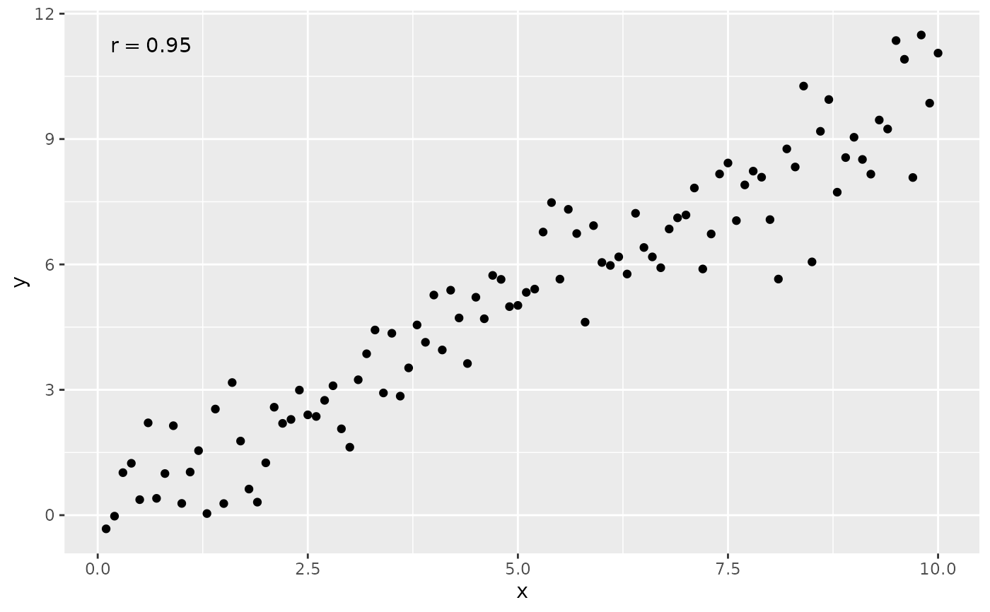
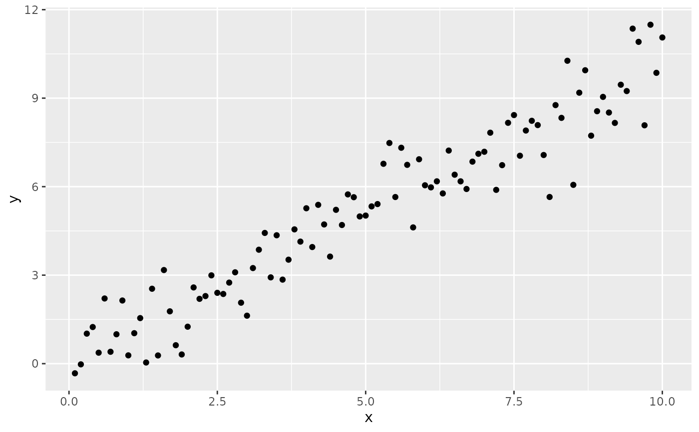
# by default only R is displayed
ggplot(my.data, aes(x, y)) +
  geom_point() +
  stat_correlation()


ggplot(my.data, aes(x, y)) +
  geom_point() +
  stat_correlation(small.r = TRUE)


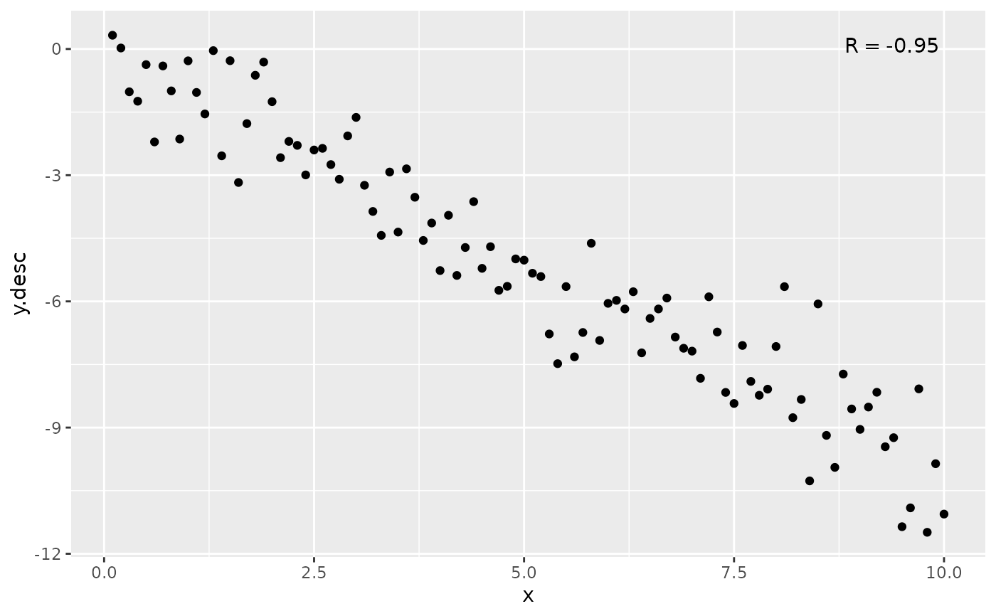
ggplot(my.data, aes(x, y.desc)) +
  geom_point() +
  stat_correlation(label.x = "right")


# non-default methods
ggplot(my.data, aes(x, y)) +
  geom_point() +
  stat_correlation(method = "kendall")


ggplot(my.data, aes(x, y)) +
  geom_point() +
  stat_correlation(method = "spearman")


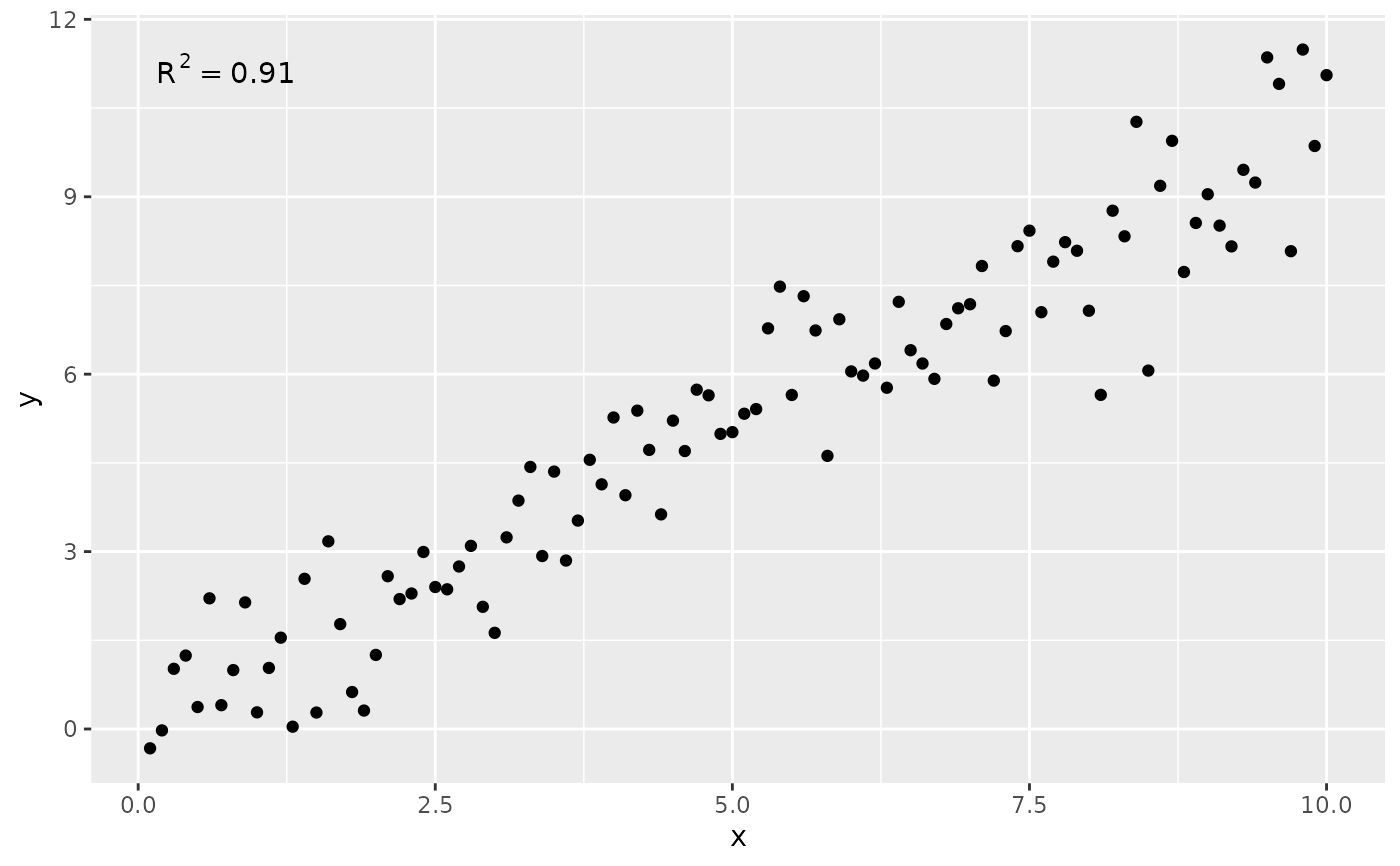
# use_label() can map a user selected label
ggplot(my.data, aes(x, y)) +
  geom_point() +
  stat_correlation(use_label("R2"))


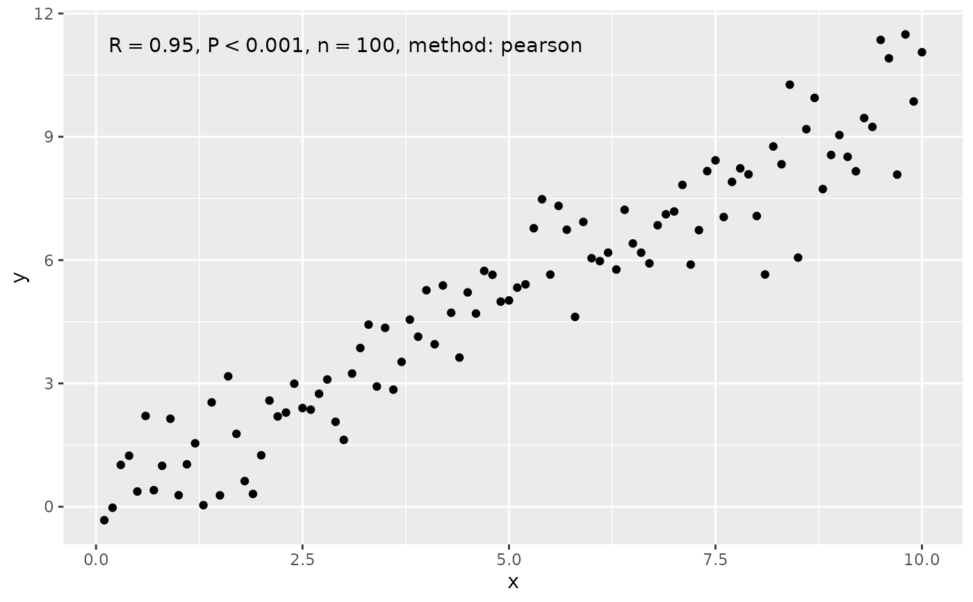
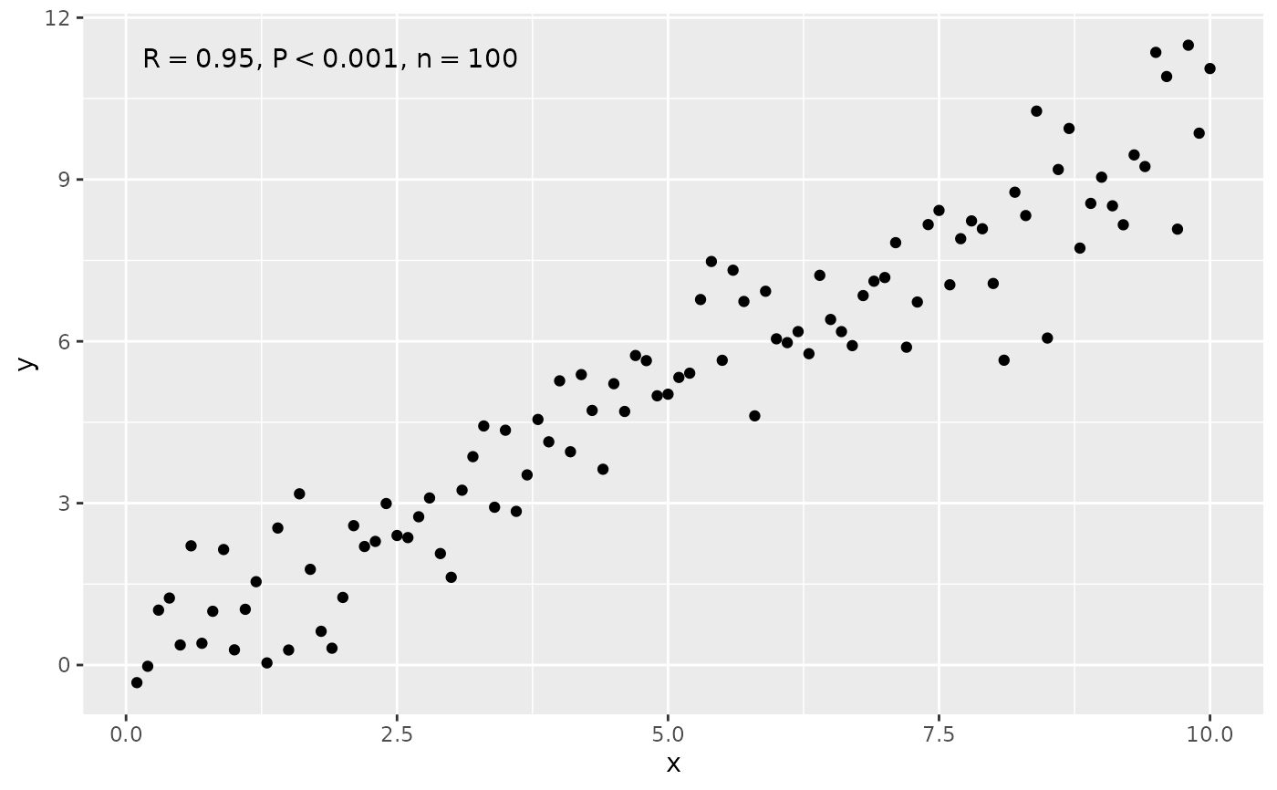
# use_label() can assemble and map a combined label
ggplot(my.data, aes(x, y)) +
  geom_point() +
  stat_correlation(use_label("R", "P", "n", "method"))


ggplot(my.data, aes(x, y)) +
  geom_point() +
  stat_correlation(use_label("R", "R.CI"))


ggplot(my.data, aes(x, y)) +
  geom_point() +
  stat_correlation(use_label("R", "R.CI"),
                   r.conf.level = 0.95)


ggplot(my.data, aes(x, y)) +
  geom_point() +
  stat_correlation(use_label("R", "R.CI"),
                   method = "kendall",
                   r.conf.level = 0.95)


ggplot(my.data, aes(x, y)) +
  geom_point() +
  stat_correlation(use_label("R", "R.CI"),
                   method = "spearman",
                   r.conf.level = 0.95)


# manually assemble and map a specific label using paste() and aes()
ggplot(my.data, aes(x, y)) +
  geom_point() +
  stat_correlation(aes(label = paste(after_stat(r.label),
                                     after_stat(p.value.label),
                                     after_stat(n.label),
                                     sep = "*\", \"*")))


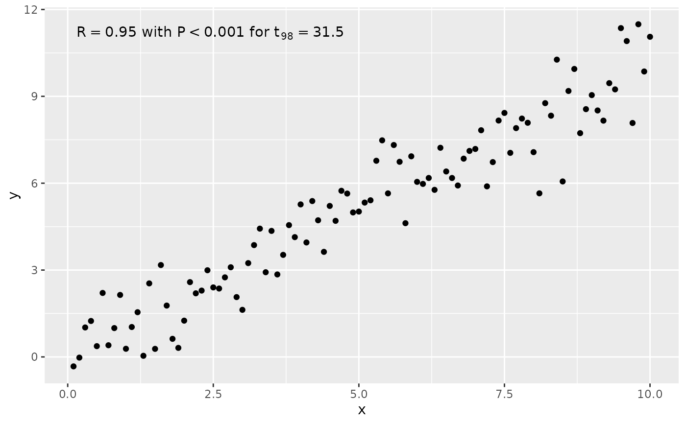
# manually format and map a specific label using sprintf() and aes()
ggplot(my.data, aes(x, y)) +
  geom_point() +
  stat_correlation(aes(label = sprintf("%s*\" with \"*%s*\" for \"*%s",
                                       after_stat(r.label),
                                       after_stat(p.value.label),
                                       after_stat(t.value.label))))


# Inspecting the returned data using geom_debug()
# This provides a quick way of finding out the names of the variables that
# are available for mapping to aesthetics with after_stat().

gginnards.installed <- requireNamespace("gginnards", quietly = TRUE)

if (gginnards.installed)
  library(gginnards)

# the whole of computed data
if (gginnards.installed)
  ggplot(my.data, aes(x, y)) +
    geom_point() +
    stat_correlation(geom = "debug")

#> [1] "PANEL 1; group(s) -1; 'draw_function()' input 'data' (head):"
#>   npcx npcy                label  t.value df      p.value       cor      test
#> 1   NA   NA italic(R)~`=`~"0.95" 31.54257 98 4.019532e-53 0.9541138 two.sided
#>     n  method r.conf.level r.confint.low r.confint.high         p.value.label
#> 1 100 pearson         0.95     0.9324397      0.9689463 italic(P)~`<`~"0.001"
#>             n.label grp.label              r.label       r.confint.label
#> 1 italic(n)~`=`~100        -1 italic(R)~`=`~"0.95" "95% CI [0.93, 0.97]"
#>        method.label            cor.label               rr.label
#> 1 "method: pearson" italic(R)~`=`~"0.95" italic(R)^2~`=`~"0.91"
#>              t.value.label   x        y PANEL group
#> 1 italic(t)[98]~`=`~"31.5" 0.1 11.48941     1    -1

if (gginnards.installed)
  ggplot(my.data, aes(x, y)) +
    geom_point() +
    stat_correlation(geom = "debug", method = "pearson")

#> [1] "PANEL 1; group(s) -1; 'draw_function()' input 'data' (head):"
#>   npcx npcy                label  t.value df      p.value       cor      test
#> 1   NA   NA italic(R)~`=`~"0.95" 31.54257 98 4.019532e-53 0.9541138 two.sided
#>     n  method r.conf.level r.confint.low r.confint.high         p.value.label
#> 1 100 pearson         0.95     0.9324397      0.9689463 italic(P)~`<`~"0.001"
#>             n.label grp.label              r.label       r.confint.label
#> 1 italic(n)~`=`~100        -1 italic(R)~`=`~"0.95" "95% CI [0.93, 0.97]"
#>        method.label            cor.label               rr.label
#> 1 "method: pearson" italic(R)~`=`~"0.95" italic(R)^2~`=`~"0.91"
#>              t.value.label   x        y PANEL group
#> 1 italic(t)[98]~`=`~"31.5" 0.1 11.48941     1    -1

if (gginnards.installed)
  ggplot(my.data, aes(x, y)) +
    geom_point() +
    stat_correlation(geom = "debug", method = "kendall")

#> [1] "PANEL 1; group(s) -1; 'draw_function()' input 'data' (head):"
#>   npcx npcy                  label  z.value      p.value       tau      test
#> 1   NA   NA italic(tau)~`=`~"0.82" 12.13285 7.074566e-34 0.8230303 two.sided
#>     n  method r.conf.level r.confint.low r.confint.high         p.value.label
#> 1 100 kendall            0            NA             NA italic(P)~`<`~"0.001"
#>             n.label grp.label                r.label r.confint.label
#> 1 italic(n)~`=`~100        -1 italic(tau)~`=`~"0.82"            <NA>
#>        method.label              tau.label tau.confint.label
#> 1 "method: kendall" italic(tau)~`=`~"0.82"              <NA>
#>          z.value.label   x        y PANEL group
#> 1 italic(z)~`=`~"12.1" 0.1 11.48941     1    -1

if (gginnards.installed)
  ggplot(my.data, aes(x, y)) +
    geom_point() +
    stat_correlation(geom = "debug", method = "spearman")

#> [1] "PANEL 1; group(s) -1; 'draw_function()' input 'data' (head):"
#>   npcx npcy                  label S.value p.value       rho      test   n
#> 1   NA   NA italic(rho)~`=`~"0.96"    6974       0 0.9581518 two.sided 100
#>     method r.conf.level r.confint.low r.confint.high         p.value.label
#> 1 spearman            0            NA             NA italic(P)~`<`~"0.001"
#>             n.label grp.label                r.label r.confint.label
#> 1 italic(n)~`=`~100        -1 italic(rho)~`=`~"0.96"            <NA>
#>         method.label              rho.label rho.confint.label
#> 1 "method: spearman" italic(rho)~`=`~"0.96"              <NA>
#>                         S.value.label   x        y PANEL group
#> 1 italic(S)~`=`~"6.97" %*% 10^{"+03"} 0.1 11.48941     1    -1

if (gginnards.installed)
  ggplot(my.data, aes(x, y)) +
    geom_point() +
    stat_correlation(geom = "debug", output.type = "numeric")

#> [1] "PANEL 1; group(s) -1; 'draw_function()' input 'data' (head):"
#>   npcx npcy label  t.value df      p.value       cor      test   n  method
#> 1   NA   NA  <NA> 31.54257 98 4.019532e-53 0.9541138 two.sided 100 pearson
#>   r.conf.level r.confint.low r.confint.high r.label   x        y PANEL group
#> 1         0.95     0.9324397      0.9689463    <NA> 0.1 11.48941     1    -1

if (gginnards.installed)
  ggplot(my.data, aes(x, y)) +
    geom_point() +
    stat_correlation(geom = "debug", output.type = "markdown")

#> [1] "PANEL 1; group(s) -1; 'draw_function()' input 'data' (head):"
#>   npcx npcy      label  t.value df      p.value       cor      test   n  method
#> 1   NA   NA _R_ = 0.95 31.54257 98 4.019532e-53 0.9541138 two.sided 100 pearson
#>   r.conf.level r.confint.low r.confint.high p.value.label   n.label grp.label
#> 1         0.95     0.9324397      0.9689463   _P_ < 0.001 _n_ = 100        -1
#>      r.label     r.confint.label      method.label  cor.label
#> 1 _R_ = 0.95 95% CI [0.93, 0.97] "method: pearson" _R_ = 0.95
#>                 rr.label           t.value.label   x        y PANEL group
#> 1 _R_<sup>2</sup> = 0.91 _t_<sub>98</sub> = 31.5 0.1 11.48941     1    -1

if (gginnards.installed)
  ggplot(my.data, aes(x, y)) +
    geom_point() +
    stat_correlation(geom = "debug", output.type = "LaTeX")

#> [1] "PANEL 1; group(s) -1; 'draw_function()' input 'data' (head):"
#>   npcx npcy    label  t.value df      p.value       cor      test   n  method
#> 1   NA   NA R = 0.95 31.54257 98 4.019532e-53 0.9541138 two.sided 100 pearson
#>   r.conf.level r.confint.low r.confint.high p.value.label           n.label
#> 1         0.95     0.9324397      0.9689463     P < 0.001 \\mathit{n} = 100
#>   grp.label  r.label     r.confint.label      method.label cor.label   rr.label
#> 1        -1 R = 0.95 95% CI [0.93, 0.97] "method: pearson"  R = 0.95 R^2 = 0.91
#>   t.value.label   x        y PANEL group
#> 1 t_{98} = 31.5 0.1 11.48941     1    -1