Plot Components of a GAM Object

A plot method for GAM objects, which can be used on GLM and LM objects as well. It focuses on terms (main-effects), and produces a suitable plot for terms of different types

Usage

# S3 method for class 'Gam'
plot(
  x,
  residuals = NULL,
  rugplot = TRUE,
  se = FALSE,
  scale = 0,
  ask = FALSE,
  terms = labels.Gam(x),
  ...
)

# S3 method for class 'Gam'
preplot(object, newdata, terms = labels.Gam(object), ...)

Arguments

x: a Gam object, or a preplot.Gam object. The first thing plot.Gam() does is check if x has a component called preplot; if not, it computes one using preplot.Gam(). Either way, it is this preplot.Gam object that is required for plotting a Gam object.
residuals: if TRUE, partial deviance residuals are plotted along with the fitted terms—default is FALSE. If residuals is a vector with the same length as each fitted term in x, then these are taken to be the overall residuals to be used for constructing the partial residuals.
rugplot: if TRUE (the default), a univariate histogram or rugplot is displayed along the base of each plot, showing the occurrence of each x; ties are broken by jittering.
se: if TRUE, upper and lower pointwise twice-standard-error curves are included for each plot. The default is FALSE.
scale: a lower limit for the number of units covered by the limits on the y for each plot. The default is scale=0, in which case each plot uses the range of the functions being plotted to create their ylim. By setting scale to be the maximum value of diff(ylim) for all the plots, then all subsequent plots will produced in the same vertical units. This is essential for comparing the importance of fitted terms in additive models.
ask: if TRUE, plot.Gam() operates in interactive mode.
terms: subsets of the terms can be selected
...: Additonal plotting arguments, not all of which will work (like xlim)
object: same as x
newdata: if supplied to preplot.Gam, the preplot object is based on them rather than the original.

Value

a plot is produced for each of the terms in the object x. The function currently knows how to plot all main-effect functions of one or two predictors. So in particular, interactions are not plotted. An appropriate x-y is produced to display each of the terms, adorned with residuals, standard-error curves, and a rugplot, depending on the choice of options. The form of the plot is different, depending on whether the x-value for each plot is numeric, a factor, or a matrix.

When ask=TRUE, rather than produce each plot sequentially, plot.Gam() displays a menu listing all the terms that can be plotted, as well as switches for all the options.

A preplot.Gam object is a list of precomputed terms. Each such term (also a preplot.Gam object) is a list with components x, y and others—the basic ingredients needed for each term plot. These are in turn handed to the specialized plotting function gplot(), which has methods for different classes of the leading x argument. In particular, a different plot is produced if x is numeric, a category or factor, a matrix, or a list. Experienced users can extend this range by creating more gplot() methods for other classes. Graphical parameters (see par) may also be supplied as arguments to this function. This function is a method for the generic function plot() for class "Gam".

It can be invoked by calling plot(x) for an object x of the appropriate class, or directly by calling plot.Gam(x) regardless of the class of the object.

References

Hastie, T. J. (1992) Generalized additive models. Chapter 7 of Statistical Models in S eds J. M. Chambers and T. J. Hastie, Wadsworth & Brooks/Cole.

Hastie, T. and Tibshirani, R. (1990) Generalized Additive Models. London: Chapman and Hall.

Author

Written by Trevor Hastie, following closely the design in the "Generalized Additive Models" chapter (Hastie, 1992) in Chambers and Hastie (1992).

Examples


data(gam.data)
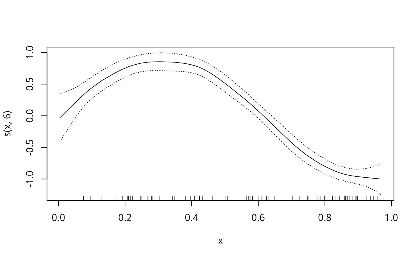
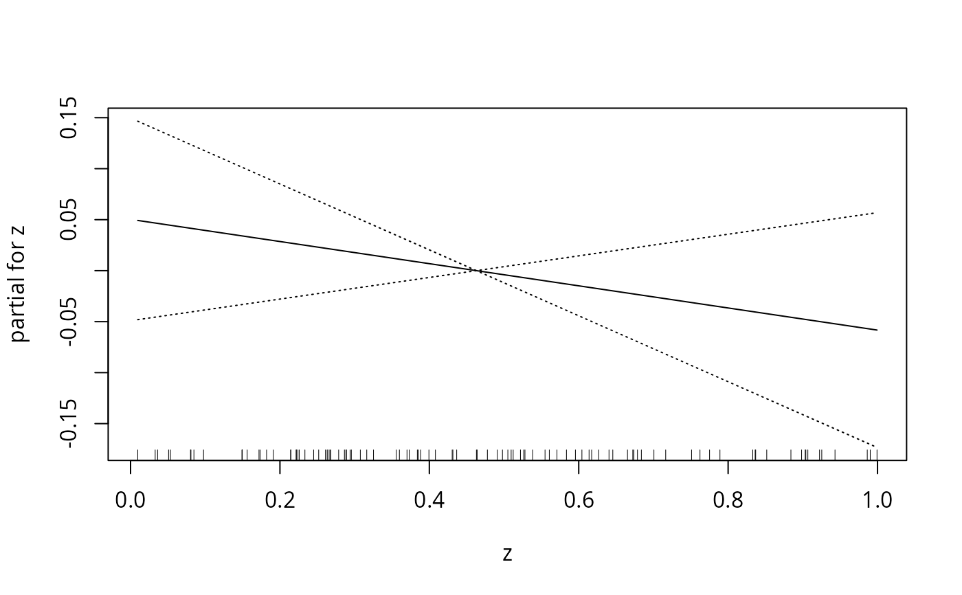
Gam.object <- gam(y ~ s(x,6) + z,data=gam.data)
plot(Gam.object,se=TRUE)


data(gam.newdata)
preplot(Gam.object,newdata=gam.newdata)
#> Warning: No standard errors (currently) for gam predictions with newdata
#> $`s(x, 6)`
#> $x
#>  [1] 0.1 0.2 0.3 0.4 0.5 0.6 0.7 0.8 0.9 1.0
#> 
#> $y
#>           1           2           3           4           5           6 
#>  0.44379143  0.75360796  0.85468111  0.80512984  0.51279094  0.07523574 
#>           7           8           9          10 
#> -0.42622549 -0.80005872 -0.96321574 -1.01594919 
#> 
#> $se.y
#> NULL
#> 
#> $xlab
#> [1] "x"
#> 
#> $ylab
#> [1] "s(x, 6)"
#> 
#> attr(,"class")
#> [1] "preplot.Gam"
#> 
#> $z
#> $x
#>  [1] 0.1 0.2 0.3 0.4 0.5 0.6 0.7 0.8 0.9 1.0
#> 
#> $y
#>            1            2            3            4            5            6 
#>  0.039428080  0.028567775  0.017707471  0.006847166 -0.004013139 -0.014873443 
#>            7            8            9           10 
#> -0.025733748 -0.036594052 -0.047454357 -0.058314661 
#> 
#> $se.y
#> NULL
#> 
#> $xlab
#> [1] "z"
#> 
#> $ylab
#> [1] "partial for z"
#> 
#> attr(,"class")
#> [1] "preplot.Gam"
#> 
#> attr(,"class")
#> [1] "preplot.Gam"