Fitting Generalized Additive Models

gam is used to fit generalized additive models, specified by giving a symbolic description of the additive predictor and a description of the error distribution. gam uses the backfitting algorithm to combine different smoothing or fitting methods. The methods currently supported are local regression and smoothing splines.

Usage

gam(
  formula,
  family = gaussian,
  data,
  weights,
  subset,
  na.action,
  start = NULL,
  etastart,
  mustart,
  control = gam.control(...),
  model = TRUE,
  method = "glm.fit",
  x = FALSE,
  y = TRUE,
  ...
)

gam.fit(
  x,
  y,
  smooth.frame,
  weights = rep(1, nobs),
  start = NULL,
  etastart = NULL,
  mustart = NULL,
  offset = rep(0, nobs),
  family = gaussian(),
  control = gam.control()
)

Arguments

formula

a formula expression as for other regression models, of the form response ~ predictors. See the documentation of lm and formula for details. Built-in nonparametric smoothing terms are indicated by s for smoothing splines or lo for loess smooth terms. See the documentation for s and lo for their arguments. Additional smoothers can be added by creating the appropriate interface functions. Interactions with nonparametric smooth terms are not fully supported, but will not produce errors; they will simply produce the usual parametric interaction.

family

a description of the error distribution and link function to be used in the model. This can be a character string naming a family function, a family function or the result of a call to a family function. (See family for details of family functions.)

data

an optional data frame containing the variables in the model. If not found in data, the variables are taken from environment(formula), typically the environment from which gam is called.

weights

an optional vector of weights to be used in the fitting process.

subset

an optional vector specifying a subset of observations to be used in the fitting process.

na.action

a function which indicates what should happen when the data contain NAs. The default is set by the na.action setting of options, and is na.fail if that is unset. The “factory-fresh” default is na.omit. A special method na.gam.replace allows for mean-imputation of missing values (assumes missing at random), and works gracefully with gam

start

starting values for the parameters in the additive predictor.

etastart

starting values for the additive predictor.

mustart

starting values for the vector of means.

control

a list of parameters for controlling the fitting process. See the documentation for gam.control for details. These can also be set as arguments to gam() itself.

model

a logical value indicating whether model frame should be included as a component of the returned value. Needed if gam is called and predicted from inside a user function. Default is TRUE.

method

the method to be used in fitting the parametric part of the model. The default method "glm.fit" uses iteratively reweighted least squares (IWLS). The only current alternative is "model.frame" which returns the model frame and does no fitting.

x, y

For gam: logical values indicating whether the response vector and model matrix used in the fitting process should be returned as components of the returned value.

For gam.fit: x is a model matrix of dimension n * p, and y is a vector of observations of length n.

...

further arguments passed to or from other methods.

smooth.frame

for gam.fit only. This is essentially a subset of the model frame corresponding to the smooth terms, and has the ingredients needed for smoothing each variable in the backfitting algorithm. The elements of this frame are produced by the formula functions lo and s.

offset

this can be used to specify an a priori known component to be included in the additive predictor during fitting.

Value

gam returns an object of class Gam, which inherits from both glm and lm.

Gam objects can be examined by print, summary, plot, and anova. Components can be extracted using extractor functions predict, fitted, residuals, deviance, formula, and family. Can be modified using update. It has all the components of a glm object, with a few more. This also means it can be queried, summarized etc by methods for glm and lm objects. Other generic functions that have methods for Gam objects are step and preplot.

The following components must be included in a legitimate `Gam' object. The residuals, fitted values, coefficients and effects should be extracted by the generic functions of the same name, rather than by the "$" operator. The family function returns the entire family object used in the fitting, and deviance can be used to extract the deviance of the fit.

coefficients: the coefficients of the parametric part of the additive.predictors, which multiply the columns of the model matrix. The names of the coefficients are the names of the single-degree-of-freedom effects (the columns of the model matrix). If the model is overdetermined there will be missing values in the coefficients corresponding to inestimable coefficients.
additive.predictors: the additive fit, given by the product of the model matrix and the coefficients, plus the columns of the $smooth component.
fitted.values: the fitted mean values, obtained by transforming the component additive.predictors using the inverse link function.
smooth, nl.df, nl.chisq, var: these four characterize the nonparametric aspect of the fit. smooth is a matrix of smooth terms, with a column corresponding to each smooth term in the model; if no smooth terms are in the Gam model, all these components will be missing. Each column corresponds to the strictly nonparametric part of the term, while the parametric part is obtained from the model matrix. nl.df is a vector giving the approximate degrees of freedom for each column of smooth. For smoothing splines specified by s(x), the approximate df will be the trace of the implicit smoother matrix minus 2. nl.chisq is a vector containing a type of score test for the removal of each of the columns of smooth. var is a matrix like smooth, containing the approximate pointwise variances for the columns of smooth.
smooth.frame: This is essentially a subset of the model frame corresponding to the smooth terms, and has the ingredients needed for making predictions from a Gam object
residuals: the residuals from the final weighted additive fit; also known as residuals, these are typically not interpretable without rescaling by the weights.
deviance: up to a constant, minus twice the maximized log-likelihood. Similar to the residual sum of squares. Where sensible, the constant is chosen so that a saturated model has deviance zero.
null.deviance: The deviance for the null model, comparable with deviance. The null model will include the offset, and an intercept if there is one in the model
iter: the number of local scoring iterations used to compute the estimates.
bf.iter: a vector of length iter giving number of backfitting iterations used at each inner loop.
family: a three-element character vector giving the name of the family, the link, and the variance function; mainly for printing purposes.
weights: the working weights, that is the weights in the final iteration of the local scoring fit.
prior.weights: the case weights initially supplied.
df.residual: the residual degrees of freedom.
df.null: the residual degrees of freedom for the null model.

The object will also have the components of a lm object: coefficients, residuals, fitted.values, call, terms, and some others involving the numerical fit. See lm.object.

Details

The gam model is fit using the local scoring algorithm, which iteratively fits weighted additive models by backfitting. The backfitting algorithm is a Gauss-Seidel method for fitting additive models, by iteratively smoothing partial residuals. The algorithm separates the parametric from the nonparametric part of the fit, and fits the parametric part using weighted linear least squares within the backfitting algorithm. This version of gam remains faithful to the philosophy of GAM models as outlined in the references below.

An object gam.slist (currently set to c("lo","s","random")) lists the smoothers supported by gam. Corresponding to each of these is a smoothing function gam.lo, gam.s etc that take particular arguments and produce particular output, custom built to serve as building blocks in the backfitting algorithm. This allows users to add their own smoothing methods. See the documentation for these methods for further information. In addition, the object gam.wlist (currently set to c("s","lo")) lists the smoothers for which efficient backfitters are provided. These are invoked if all the smoothing methods are of one kind (either all "lo" or all "s").

References

Hastie, T. J. (1991) Generalized additive models. Chapter 7 of Statistical Models in S eds J. M. Chambers and T. J. Hastie, Wadsworth & Brooks/Cole.

Hastie, T. and Tibshirani, R. (1990) Generalized Additive Models. London: Chapman and Hall.

Venables, W. N. and Ripley, B. D. (2002) Modern Applied Statistics with S. New York: Springer.

Author

Written by Trevor Hastie, following closely the design in the "Generalized Additive Models" chapter (Hastie, 1992) in Chambers and Hastie (1992), and the philosophy in Hastie and Tibshirani (1991). This version of gam is adapted from the S version to match the glm and lm functions in R.

Note that this version of gam is different from the function with the same name in the R library mgcv, which uses only smoothing splines with a focus on automatic smoothing parameter selection via GCV. To avoid issues with S3 method handling when both packages are loaded, the object class in package "gam" is now "Gam".

Examples


data(kyphosis)
gam(Kyphosis ~ s(Age,4) + Number, family = binomial, data=kyphosis,
trace=TRUE)
#> GAM s.wam loop 1: deviance = 66.42095 
#> GAM s.wam loop 2: deviance = 63.77252 
#> GAM s.wam loop 3: deviance = 63.25199 
#> GAM s.wam loop 4: deviance = 63.13399 
#> GAM s.wam loop 5: deviance = 63.11016 
#> GAM s.wam loop 6: deviance = 63.10748 
#> GAM s.wam loop 7: deviance = 63.10727 
#> GAM s.wam loop 8: deviance = 63.10725 
#> GAM s.wam loop 9: deviance = 63.10725 
#> Call:
#> gam(formula = Kyphosis ~ s(Age, 4) + Number, family = binomial, 
#>     data = kyphosis, trace = TRUE)
#> 
#> Degrees of Freedom: 80 total; 75.00002 Residual
#> Residual Deviance: 63.10725 
data(airquality)
gam(Ozone^(1/3) ~ lo(Solar.R) + lo(Wind, Temp), data=airquality, na=na.gam.replace)
#> Warning: 37 observations omitted due to missing values in the response
#> Call:
#> gam(formula = Ozone^(1/3) ~ lo(Solar.R) + lo(Wind, Temp), data = airquality, 
#>     na.action = na.gam.replace)
#> 
#> Degrees of Freedom: 115 total; 102.6679 Residual
#> Residual Deviance: 20.05229 
gam(Kyphosis ~ poly(Age,2) + s(Start), data=kyphosis, family=binomial, subset=Number>2)
#> Call:
#> gam(formula = Kyphosis ~ poly(Age, 2) + s(Start), family = binomial, 
#>     data = kyphosis, subset = Number > 2)
#> 
#> Degrees of Freedom: 68 total; 61.99976 Residual
#> Residual Deviance: 44.5635 
data(gam.data)
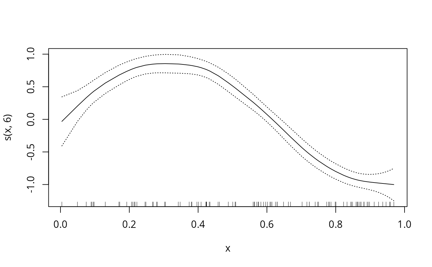
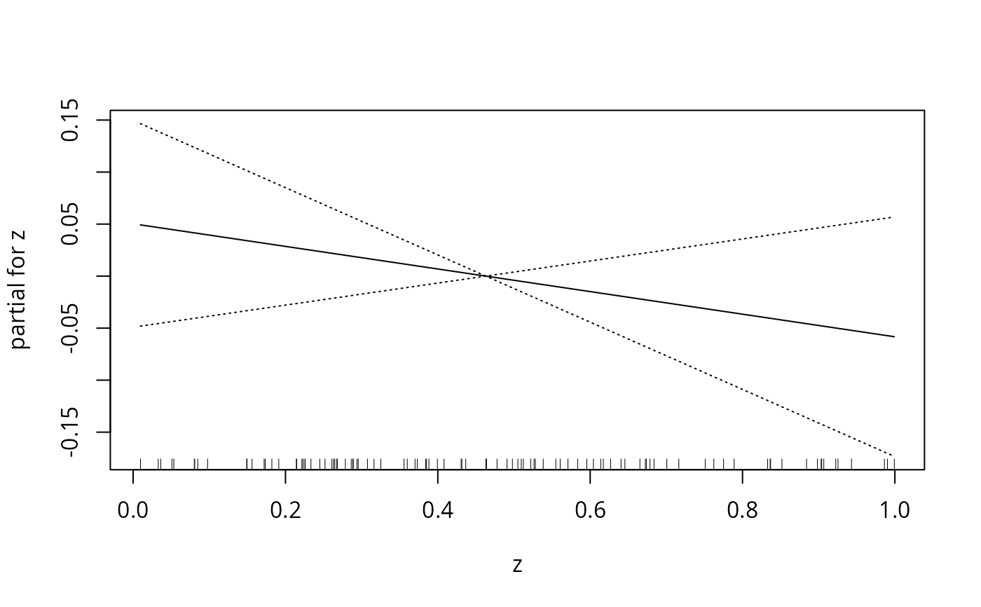
Gam.object <- gam(y ~ s(x,6) + z,data=gam.data)
summary(Gam.object)
#> 
#> Call: gam(formula = y ~ s(x, 6) + z, data = gam.data)
#> Deviance Residuals:
#>      Min       1Q   Median       3Q      Max 
#> -0.59177 -0.18050  0.01291  0.23941  0.51412 
#> 
#> (Dispersion Parameter for gaussian family taken to be 0.0823)
#> 
#>     Null Deviance: 57.7496 on 99 degrees of freedom
#> Residual Deviance: 7.5745 on 92.0003 degrees of freedom
#> AIC: 43.7495 
#> 
#> Number of Local Scoring Iterations: NA 
#> 
#> Anova for Parametric Effects
#>           Df Sum Sq Mean Sq  F value Pr(>F)    
#> s(x, 6)    1 38.210  38.210 464.0987 <2e-16 ***
#> z          1  0.084   0.084   1.0247 0.3141    
#> Residuals 92  7.575   0.082                    
#> ---
#> Signif. codes:  0 ‘***’ 0.001 ‘**’ 0.01 ‘*’ 0.05 ‘.’ 0.1 ‘ ’ 1
#> 
#> Anova for Nonparametric Effects
#>             Npar Df Npar F     Pr(F)    
#> (Intercept)                             
#> s(x, 6)           5 28.697 < 2.2e-16 ***
#> z                                       
#> ---
#> Signif. codes:  0 ‘***’ 0.001 ‘**’ 0.01 ‘*’ 0.05 ‘.’ 0.1 ‘ ’ 1
plot(Gam.object,se=TRUE)


data(gam.newdata)
predict(Gam.object,type="terms",newdata=gam.newdata)
#>        s(x, 6)            z
#> 1   0.44379143  0.039428080
#> 2   0.75360796  0.028567775
#> 3   0.85468111  0.017707471
#> 4   0.80512984  0.006847166
#> 5   0.51279094 -0.004013139
#> 6   0.07523574 -0.014873443
#> 7  -0.42622549 -0.025733748
#> 8  -0.80005872 -0.036594052
#> 9  -0.96321574 -0.047454357
#> 10 -1.01594919 -0.058314661
#> attr(,"constant")
#> [1] 0.634896