Gap Statistic for Estimating the Number of Clusters
clusGap.RdclusGap() calculates a goodness of clustering measure, the
“gap” statistic. For each number of clusters \(k\), it
compares \(\log(W(k))\) with
\(E^*[\log(W(k))]\) where the latter is defined via
bootstrapping, i.e., simulating from a reference (\(H_0\))
distribution, a uniform distribution on the hypercube determined by
the ranges of x, after first centering, and then
svd (aka ‘PCA’)-rotating them when (as by
default) spaceH0 = "scaledPCA".
maxSE(f, SE.f) determines the location of the maximum
of f, taking a “1-SE rule” into account for the
*SE* methods. The default method "firstSEmax" looks for
the smallest \(k\) such that its value \(f(k)\) is not more than 1
standard error away from the first local maximum.
This is similar but not the same as "Tibs2001SEmax", Tibshirani
et al's recommendation of determining the number of clusters from the
gap statistics and their standard deviations.
Usage
clusGap(x, FUNcluster, K.max, B = 100, d.power = 1,
        spaceH0 = c("scaledPCA", "original"),
        verbose = interactive(), ...)

maxSE(f, SE.f,
      method = c("firstSEmax", "Tibs2001SEmax", "globalSEmax",
                 "firstmax", "globalmax"),
      SE.factor = 1)

# S3 method for class 'clusGap'
print(x, method = "firstSEmax", SE.factor = 1, ...)

# S3 method for class 'clusGap'
plot(x, type = "b", xlab = "k", ylab = expression(Gap[k]),
     main = NULL, do.arrows = TRUE,
     arrowArgs = list(col="red3", length=1/16, angle=90, code=3), ...)
Arguments
- x
numeric matrix or
data.frame.- FUNcluster
a
functionwhich accepts as first argument a (data) matrix likex, second argument, say \(k, k\geq 2\), the number of clusters desired, and returns alistwith a component named (or shortened to)clusterwhich is a vector of lengthn = nrow(x)of integers in1:kdetermining the clustering or grouping of thenobservations.- K.max
the maximum number of clusters to consider, must be at least two.
- B
integer, number of Monte Carlo (“bootstrap”) samples.
- d.power
a positive integer specifying the power \(p\) which is applied to the euclidean distances (
dist) before they are summed up to give \(W(k)\). The default,d.power = 1, corresponds to the “historical” R implementation, whereasd.power = 2corresponds to what Tibshirani et al had proposed. This was found by Juan Gonzalez, in 2016-02.
- spaceH0
a
characterstring specifying the space of the \(H_0\) distribution (of no cluster). Both"scaledPCA"and"original"use a uniform distribution in a hyper cube and had been mentioned in the reference;"original"been added after a proposal (including code) by Juan Gonzalez.- verbose
integer or logical, determining if “progress” output should be printed. The default prints one bit per bootstrap sample.
- ...
(for
clusGap():) optionally further arguments forFUNcluster(), seekmeansexample below.- f
numeric vector of ‘function values’, of length \(K\), whose (“1 SE respected”) maximum we want.
- SE.f
numeric vector of length \(K\) of standard errors of
f.- method
character string indicating how the “optimal” number of clusters, \(\hat k\), is computed from the gap statistics (and their standard deviations), or more generally how the location \(\hat k\) of the maximum of \(f_k\) should be determined.
"globalmax":simply corresponds to the global maximum, i.e., is
which.max(f)"firstmax":gives the location of the first local maximum.
"Tibs2001SEmax":uses the criterion, Tibshirani et al (2001) proposed: “the smallest \(k\) such that \(f(k) \ge f(k+1) - s_{k+1}\)”. Note that this chooses \(k = 1\) when all standard deviations are larger than the differences \(f(k+1) - f(k)\).
"firstSEmax":location of the first \(f()\) value which is not smaller than the first local maximum minus
SE.factor * SE.f[], i.e, within an “f S.E.” range of that maximum (see alsoSE.factor).This, the default, has been proposed by Martin Maechler in 2012, when adding
clusGap()to the cluster package, after having seen the"globalSEmax"proposal (in code) and read the"Tibs2001SEmax"proposal."globalSEmax":(used in Dudoit and Fridlyand (2002), supposedly following Tibshirani's proposition): location of the first \(f()\) value which is not smaller than the global maximum minus
SE.factor * SE.f[], i.e, within an “f S.E.” range of that maximum (see alsoSE.factor).
See the examples for a comparison in a simple case.
- SE.factor
[When
methodcontains"SE"] Determining the optimal number of clusters, Tibshirani et al. proposed the “1 S.E.”-rule. Using anSE.factor\(f\), the “f S.E.”-rule is used, more generally.
- type, xlab, ylab, main
arguments with the same meaning as in
plot.default(), with different default.- do.arrows
logical indicating if (1 SE -)“error bars” should be drawn, via
arrows().- arrowArgs
a list of arguments passed to
arrows(); the default, notablyangleandcode, provide a style matching usual error bars.
Details
The main result <res>$Tab[,"gap"] of course is from
bootstrapping aka Monte Carlo simulation and hence random, or
equivalently, depending on the initial random seed (see
set.seed()).
On the other hand, in our experience, using B = 500 gives
quite precise results such that the gap plot is basically unchanged
after an another run.
Value
clusGap(..) returns an object of S3 class "clusGap",
basically a list with components
- Tab
a matrix with
K.maxrows and 4 columns, named "logW", "E.logW", "gap", and "SE.sim", wheregap = E.logW - logW, andSE.simcorresponds to the standard error ofgap,SE.sim[k]=\(s_k\), where \(s_k := \sqrt{1 + 1/B} sd^*(gap_j)\), and \(sd^*()\) is the standard deviation of the simulated (“bootstrapped”) gap values.- call
the
clusGap(..)call.- spaceH0
the
spaceH0argument (match.arg()ed).- n
number of observations, i.e.,
nrow(x).- B
input
B- FUNcluster
input function
FUNcluster
References
Tibshirani, R., Walther, G. and Hastie, T. (2001). Estimating the number of data clusters via the Gap statistic. Journal of the Royal Statistical Society B, 63, 411–423.
Tibshirani, R., Walther, G. and Hastie, T. (2000). Estimating the number of clusters in a dataset via the Gap statistic. Technical Report. Stanford.
Dudoit, S. and Fridlyand, J. (2002) A prediction-based resampling method for estimating the number of clusters in a dataset. Genome Biology 3(7). doi:10.1186/gb-2002-3-7-research0036
Per Broberg (2006). SAGx: Statistical Analysis of the GeneChip. R package version 1.9.7. https://bioconductor.org/packages/3.12/bioc/html/SAGx.html Deprecated and removed from Bioc ca. 2022
Author
This function is originally based on the functions gap of
former (Bioconductor) package SAGx by Per Broberg,
gapStat() from former package SLmisc by Matthias Kohl
and ideas from gap() and its methods of package lga by
Justin Harrington.
The current implementation is by Martin Maechler.
The implementation of spaceH0 = "original" is based on code
proposed by Juan Gonzalez.
See also
silhouette for a much simpler less sophisticated
goodness of clustering measure.
cluster.stats() in package fpc for
alternative measures.
Examples
### --- maxSE() methods -------------------------------------------
(mets <- eval(formals(maxSE)$method))
#> [1] "firstSEmax" "Tibs2001SEmax" "globalSEmax" "firstmax"
#> [5] "globalmax"
fk <- c(2,3,5,4,7,8,5,4)
sk <- c(1,1,2,1,1,3,1,1)/2
## use plot.clusGap():
plot(structure(class="clusGap", list(Tab = cbind(gap=fk, SE.sim=sk))))
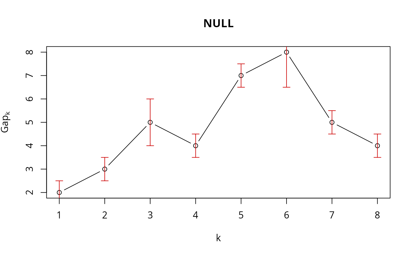 ## Note that 'firstmax' and 'globalmax' are always at 3 and 6 :
sapply(c(1/4, 1,2,4), function(SEf)
sapply(mets, function(M) maxSE(fk, sk, method = M, SE.factor = SEf)))
#> [,1] [,2] [,3] [,4]
#> firstSEmax 3 3 2 1
#> Tibs2001SEmax 3 3 1 1
#> globalSEmax 6 5 3 1
#> firstmax 3 3 3 3
#> globalmax 6 6 6 6
### --- clusGap() -------------------------------------------------
## ridiculously nicely separated clusters in 3 D :
x <- rbind(matrix(rnorm(150, sd = 0.1), ncol = 3),
matrix(rnorm(150, mean = 1, sd = 0.1), ncol = 3),
matrix(rnorm(150, mean = 2, sd = 0.1), ncol = 3),
matrix(rnorm(150, mean = 3, sd = 0.1), ncol = 3))
## Slightly faster way to use pam (see below)
pam1 <- function(x,k) list(cluster = pam(x,k, cluster.only=TRUE))
## We do not recommend using hier.clustering here, but if you want,
## there is factoextra::hcut () or a cheap version of it
hclusCut <- function(x, k, d.meth = "euclidean", ...)
list(cluster = cutree(hclust(dist(x, method=d.meth), ...), k=k))
## You can manually set it before running this : doExtras <- TRUE # or FALSE
if(!(exists("doExtras") && is.logical(doExtras)))
doExtras <- cluster:::doExtras()
if(doExtras) {
## Note we use B = 60 in the following examples to keep them "speedy".
## ---- rather keep the default B = 500 for your analysis!
## note we can pass 'nstart = 20' to kmeans() :
gskmn <- clusGap(x, FUNcluster = kmeans, nstart = 20, K.max = 8, B = 60)
gskmn #-> its print() method
plot(gskmn, main = "clusGap(., FUNcluster = kmeans, n.start=20, B= 60)")
set.seed(12); system.time(
gsPam0 <- clusGap(x, FUNcluster = pam, K.max = 8, B = 60)
)
set.seed(12); system.time(
gsPam1 <- clusGap(x, FUNcluster = pam1, K.max = 8, B = 60)
)
## and show that it gives the "same":
not.eq <- c("call", "FUNcluster"); n <- names(gsPam0)
eq <- n[!(n %in% not.eq)]
stopifnot(identical(gsPam1[eq], gsPam0[eq]))
print(gsPam1, method="globalSEmax")
print(gsPam1, method="globalmax")
print(gsHc <- clusGap(x, FUNcluster = hclusCut, K.max = 8, B = 60))
}# end {doExtras}
gs.pam.RU <- clusGap(ruspini, FUNcluster = pam1, K.max = 8, B = 60)
gs.pam.RU
#> Clustering Gap statistic ["clusGap"] from call:
#> clusGap(x = ruspini, FUNcluster = pam1, K.max = 8, B = 60)
#> B=60 simulated reference sets, k = 1..8; spaceH0="scaledPCA"
#> --> Number of clusters (method 'firstSEmax', SE.factor=1): 4
#> logW E.logW gap SE.sim
#> [1,] 7.187997 7.136220 -0.05177644 0.03256557
#> [2,] 6.628498 6.782703 0.15420450 0.03188402
#> [3,] 6.261660 6.569549 0.30788924 0.03866429
#> [4,] 5.692736 6.383480 0.69074344 0.04079079
#> [5,] 5.580999 6.229789 0.64879012 0.03871970
#> [6,] 5.500583 6.120868 0.62028520 0.03598881
#> [7,] 5.394195 6.013821 0.61962626 0.03917695
#> [8,] 5.320052 5.918920 0.59886841 0.03771544
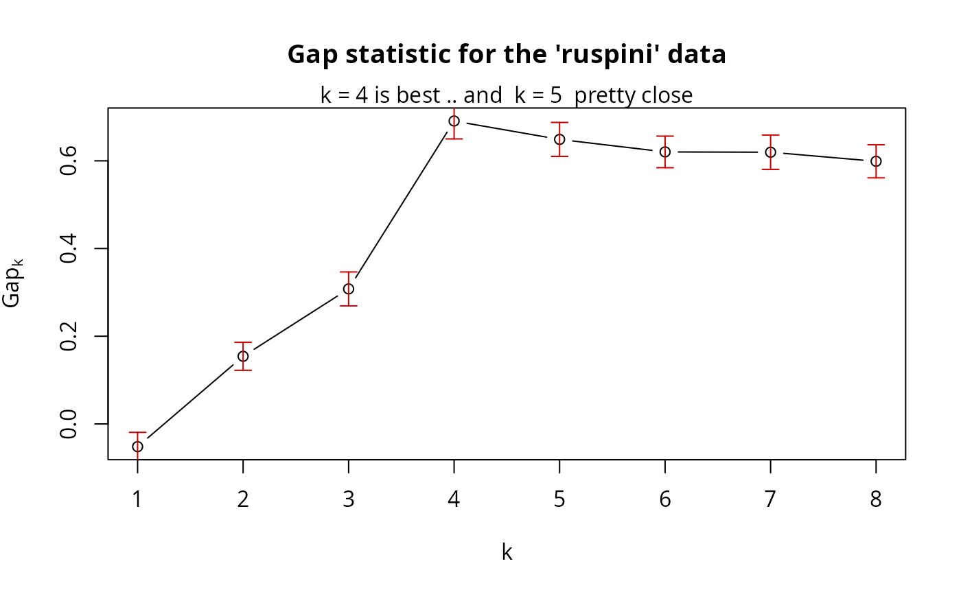
plot(gs.pam.RU, main = "Gap statistic for the 'ruspini' data")
mtext("k = 4 is best .. and k = 5 pretty close")
## Note that 'firstmax' and 'globalmax' are always at 3 and 6 :
sapply(c(1/4, 1,2,4), function(SEf)
sapply(mets, function(M) maxSE(fk, sk, method = M, SE.factor = SEf)))
#> [,1] [,2] [,3] [,4]
#> firstSEmax 3 3 2 1
#> Tibs2001SEmax 3 3 1 1
#> globalSEmax 6 5 3 1
#> firstmax 3 3 3 3
#> globalmax 6 6 6 6
### --- clusGap() -------------------------------------------------
## ridiculously nicely separated clusters in 3 D :
x <- rbind(matrix(rnorm(150, sd = 0.1), ncol = 3),
matrix(rnorm(150, mean = 1, sd = 0.1), ncol = 3),
matrix(rnorm(150, mean = 2, sd = 0.1), ncol = 3),
matrix(rnorm(150, mean = 3, sd = 0.1), ncol = 3))
## Slightly faster way to use pam (see below)
pam1 <- function(x,k) list(cluster = pam(x,k, cluster.only=TRUE))
## We do not recommend using hier.clustering here, but if you want,
## there is factoextra::hcut () or a cheap version of it
hclusCut <- function(x, k, d.meth = "euclidean", ...)
list(cluster = cutree(hclust(dist(x, method=d.meth), ...), k=k))
## You can manually set it before running this : doExtras <- TRUE # or FALSE
if(!(exists("doExtras") && is.logical(doExtras)))
doExtras <- cluster:::doExtras()
if(doExtras) {
## Note we use B = 60 in the following examples to keep them "speedy".
## ---- rather keep the default B = 500 for your analysis!
## note we can pass 'nstart = 20' to kmeans() :
gskmn <- clusGap(x, FUNcluster = kmeans, nstart = 20, K.max = 8, B = 60)
gskmn #-> its print() method
plot(gskmn, main = "clusGap(., FUNcluster = kmeans, n.start=20, B= 60)")
set.seed(12); system.time(
gsPam0 <- clusGap(x, FUNcluster = pam, K.max = 8, B = 60)
)
set.seed(12); system.time(
gsPam1 <- clusGap(x, FUNcluster = pam1, K.max = 8, B = 60)
)
## and show that it gives the "same":
not.eq <- c("call", "FUNcluster"); n <- names(gsPam0)
eq <- n[!(n %in% not.eq)]
stopifnot(identical(gsPam1[eq], gsPam0[eq]))
print(gsPam1, method="globalSEmax")
print(gsPam1, method="globalmax")
print(gsHc <- clusGap(x, FUNcluster = hclusCut, K.max = 8, B = 60))
}# end {doExtras}
gs.pam.RU <- clusGap(ruspini, FUNcluster = pam1, K.max = 8, B = 60)
gs.pam.RU
#> Clustering Gap statistic ["clusGap"] from call:
#> clusGap(x = ruspini, FUNcluster = pam1, K.max = 8, B = 60)
#> B=60 simulated reference sets, k = 1..8; spaceH0="scaledPCA"
#> --> Number of clusters (method 'firstSEmax', SE.factor=1): 4
#> logW E.logW gap SE.sim
#> [1,] 7.187997 7.136220 -0.05177644 0.03256557
#> [2,] 6.628498 6.782703 0.15420450 0.03188402
#> [3,] 6.261660 6.569549 0.30788924 0.03866429
#> [4,] 5.692736 6.383480 0.69074344 0.04079079
#> [5,] 5.580999 6.229789 0.64879012 0.03871970
#> [6,] 5.500583 6.120868 0.62028520 0.03598881
#> [7,] 5.394195 6.013821 0.61962626 0.03917695
#> [8,] 5.320052 5.918920 0.59886841 0.03771544
plot(gs.pam.RU, main = "Gap statistic for the 'ruspini' data")
mtext("k = 4 is best .. and k = 5 pretty close")
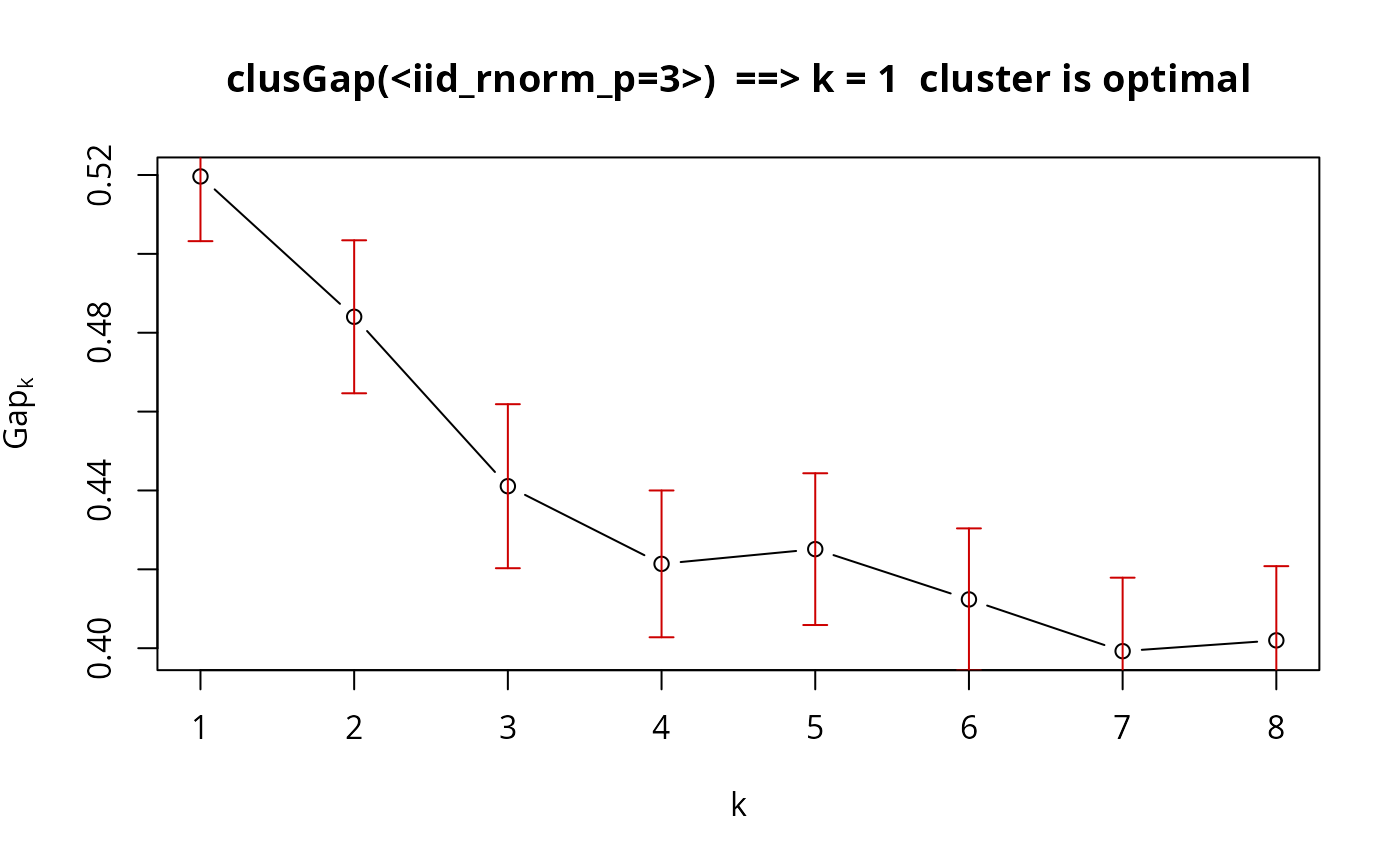
 ## This takes a minute..
## No clustering ==> k = 1 ("one cluster") should be optimal:
Z <- matrix(rnorm(256*3), 256,3)
gsP.Z <- clusGap(Z, FUNcluster = pam1, K.max = 8, B = 200)
plot(gsP.Z, main = "clusGap(<iid_rnorm_p=3>) ==> k = 1 cluster is optimal")
## This takes a minute..
## No clustering ==> k = 1 ("one cluster") should be optimal:
Z <- matrix(rnorm(256*3), 256,3)
gsP.Z <- clusGap(Z, FUNcluster = pam1, K.max = 8, B = 200)
plot(gsP.Z, main = "clusGap(<iid_rnorm_p=3>) ==> k = 1 cluster is optimal")
 gsP.Z
#> Clustering Gap statistic ["clusGap"] from call:
#> clusGap(x = Z, FUNcluster = pam1, K.max = 8, B = 200)
#> B=200 simulated reference sets, k = 1..8; spaceH0="scaledPCA"
#> --> Number of clusters (method 'firstSEmax', SE.factor=1): 1
#> logW E.logW gap SE.sim
#> [1,] 4.925966 5.445603 0.5196369 0.01641467
#> [2,] 4.779767 5.263811 0.4840440 0.01939846
#> [3,] 4.681221 5.122303 0.4410813 0.02079762
#> [4,] 4.593832 5.015217 0.4213852 0.01861287
#> [5,] 4.499340 4.924462 0.4251219 0.01924252
#> [6,] 4.431696 4.844067 0.4123709 0.01801176
#> [7,] 4.378171 4.777419 0.3992474 0.01863508
#> [8,] 4.317779 4.719767 0.4019879 0.01881713
gsP.Z
#> Clustering Gap statistic ["clusGap"] from call:
#> clusGap(x = Z, FUNcluster = pam1, K.max = 8, B = 200)
#> B=200 simulated reference sets, k = 1..8; spaceH0="scaledPCA"
#> --> Number of clusters (method 'firstSEmax', SE.factor=1): 1
#> logW E.logW gap SE.sim
#> [1,] 4.925966 5.445603 0.5196369 0.01641467
#> [2,] 4.779767 5.263811 0.4840440 0.01939846
#> [3,] 4.681221 5.122303 0.4410813 0.02079762
#> [4,] 4.593832 5.015217 0.4213852 0.01861287
#> [5,] 4.499340 4.924462 0.4251219 0.01924252
#> [6,] 4.431696 4.844067 0.4123709 0.01801176
#> [7,] 4.378171 4.777419 0.3992474 0.01863508
#> [8,] 4.317779 4.719767 0.4019879 0.01881713