Spread-Level Plots

Creates plots for examining the possible dependence of spread on level, or an extension of these plots to the studentized residuals from linear models.

Usage

spreadLevelPlot(x, ...)

slp(...)

# S3 method for class 'formula'
spreadLevelPlot(x, data=NULL, subset, na.action, 
    main=paste("Spread-Level Plot for", varnames[response], 
    "by", varnames[-response]), ...)

# Default S3 method
spreadLevelPlot(x, by, robust.line=TRUE, 
  start=0, xlab="Median", ylab="Hinge-Spread", 
  point.labels=TRUE, las=par("las"),
  main=paste("Spread-Level Plot for", deparse(substitute(x)), 
    "by", deparse(substitute(by))), 
  col=carPalette()[1], col.lines=carPalette()[2],
    pch=1, lwd=2, grid=TRUE, ...)

# S3 method for class 'lm'
spreadLevelPlot(x, robust.line=TRUE, 
  xlab="Fitted Values", ylab="Absolute Studentized Residuals", las=par("las"),
  main=paste("Spread-Level Plot for\n", deparse(substitute(x))),
  pch=1, col=carPalette()[1], col.lines=carPalette()[2:3], lwd=2, grid=TRUE, 
    id=FALSE, smooth=TRUE, ...)
    
# S3 method for class 'spreadLevelPlot'
print(x, ...)

Arguments

x: a formula of the form y ~ x, where y is a numeric vector and x is a factor, or an lm object to be plotted; alternatively a numeric vector.
data: an optional data frame containing the variables to be plotted. By default the variables are taken from the environment from which spreadLevelPlot is called.
subset: an optional vector specifying a subset of observations to be used.
na.action: a function that indicates what should happen when the data contain NAs. The default is set by the na.action setting of options.
by: a factor, numeric vector, or character vector defining groups.
robust.line: if TRUE a robust line is fit using the rlm function in the MASS package; if FALSE a line is fit using lm.
start: add the constant start to each data value.
main: title for the plot.
xlab: label for horizontal axis.
ylab: label for vertical axis.
point.labels: if TRUE label the points in the plot with group names.
las: if 0, ticks labels are drawn parallel to the axis; set to 1 for horizontal labels (see par).
col: color for points; the default is the first entry in the current car palette (see carPalette and par).
col.lines: for the default method, the line color, defaulting to the second entry in the car color palette; for the "lm" method, a vector of two colors for, respectively, the fitted straight line and a nonparametric regression smooth line, default to the second and third entries in the car color palette.
pch: plotting character for points; default is 1 (a circle, see par).
lwd: line width; default is 2 (see par).
grid: If TRUE, the default, a light-gray background grid is put on the graph
id: controls point identification; if FALSE (the default), no points are identified; can be a list of named arguments to the showLabels function; TRUE is equivalent to list(method=list("x", "y"), n=2, cex=1, col=carPalette()[1], location="lr"), which identifies the 2 points the most extreme horizontal ("X", absolute studentized residual) values and the 2 points with the most extreme horizontal ("Y", fitted values) values.
smooth: specifies the smoother to be used along with its arguments; if FALSE, no smoother is shown; can be a list giving the smoother function and its named arguments; TRUE, the default, is equivalent to list(smoother=loessLine). See ScatterplotSmoothers for the smoothers supplied by the car package and their arguments.
...: arguments passed to plotting functions.

Details

Except for linear models, computes the statistics for, and plots, a Tukey spread-level plot of log(hinge-spread) vs. log(median) for the groups; fits a line to the plot; and calculates a spread-stabilizing transformation from the slope of the line.

For linear models, plots log(abs(studentized residuals) vs. log(fitted values). Point labeling was added in November, 2016.

The function slp is an abbreviation for spreadLevelPlot.

Value

An object of class spreadLevelPlot containing:

Statistics: a matrix with the lower-hinge, median, upper-hinge, and hinge-spread for each group. (Not for an lm object.)
PowerTransformation: spread-stabilizing power transformation, calculated as \(1 - slope\) of the line fit to the plot.

References

Fox, J. (2016) Applied Regression Analysis and Generalized Linear Models, Third Edition. Sage.

Fox, J. and Weisberg, S. (2019) An R Companion to Applied Regression, Third Edition, Sage.

Hoaglin, D. C., Mosteller, F. and Tukey, J. W. (Eds.) (1983) Understanding Robust and Exploratory Data Analysis. Wiley.

Author

John Fox jfox@mcmaster.ca

Examples

spreadLevelPlot(interlocks + 1 ~ nation, data=Ornstein)

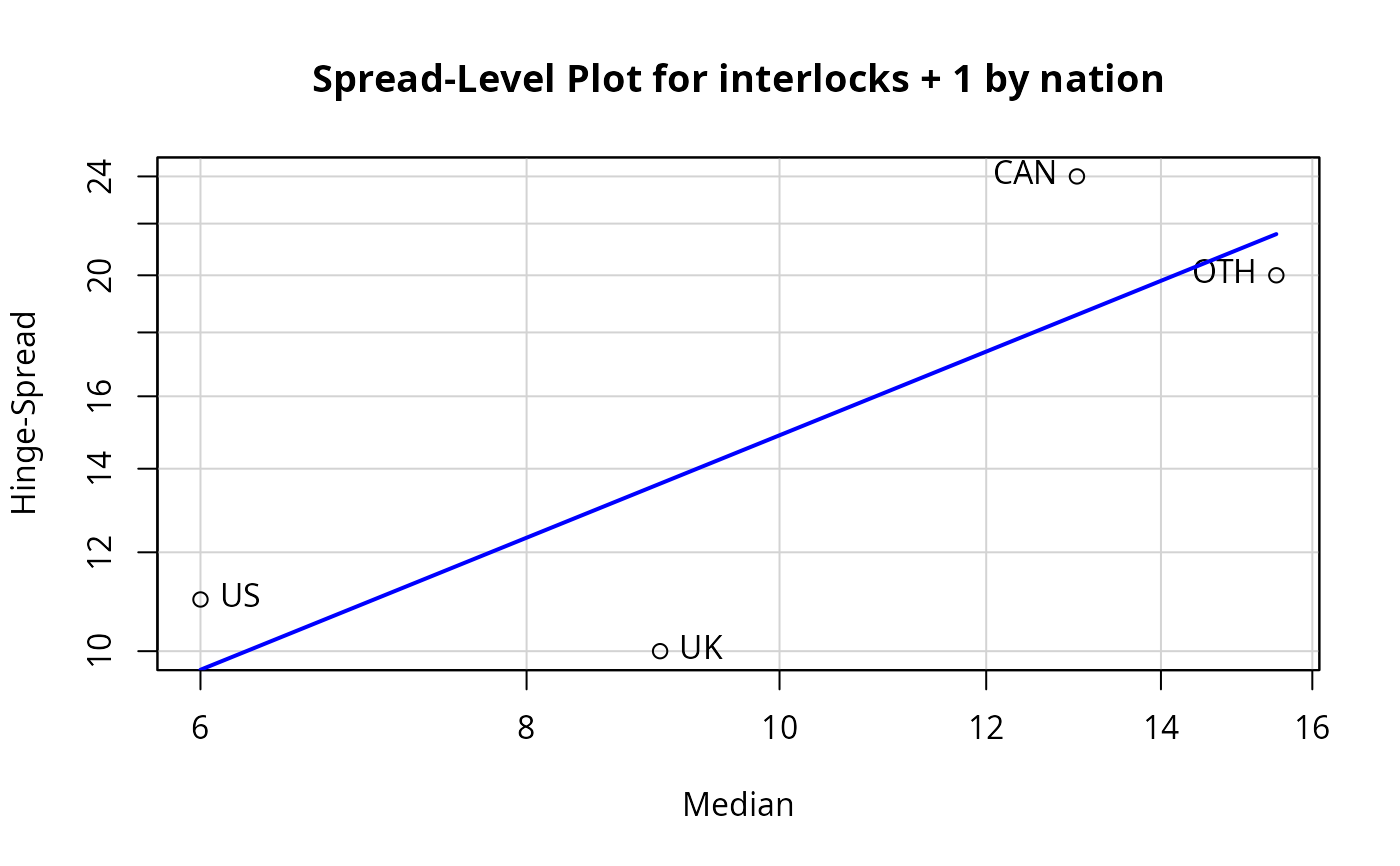#>     LowerHinge Median UpperHinge Hinge-Spread
#> US           2    6.0         13           11
#> UK           4    9.0         14           10
#> CAN          6   13.0         30           24
#> OTH          4   15.5         24           20
#> 
#> Suggested power transformation:  0.1534487 
slp(lm(interlocks + 1 ~ assets + sector + nation, data=Ornstein))
#> Warning: 
#> 1 negative fitted value removed

#> 
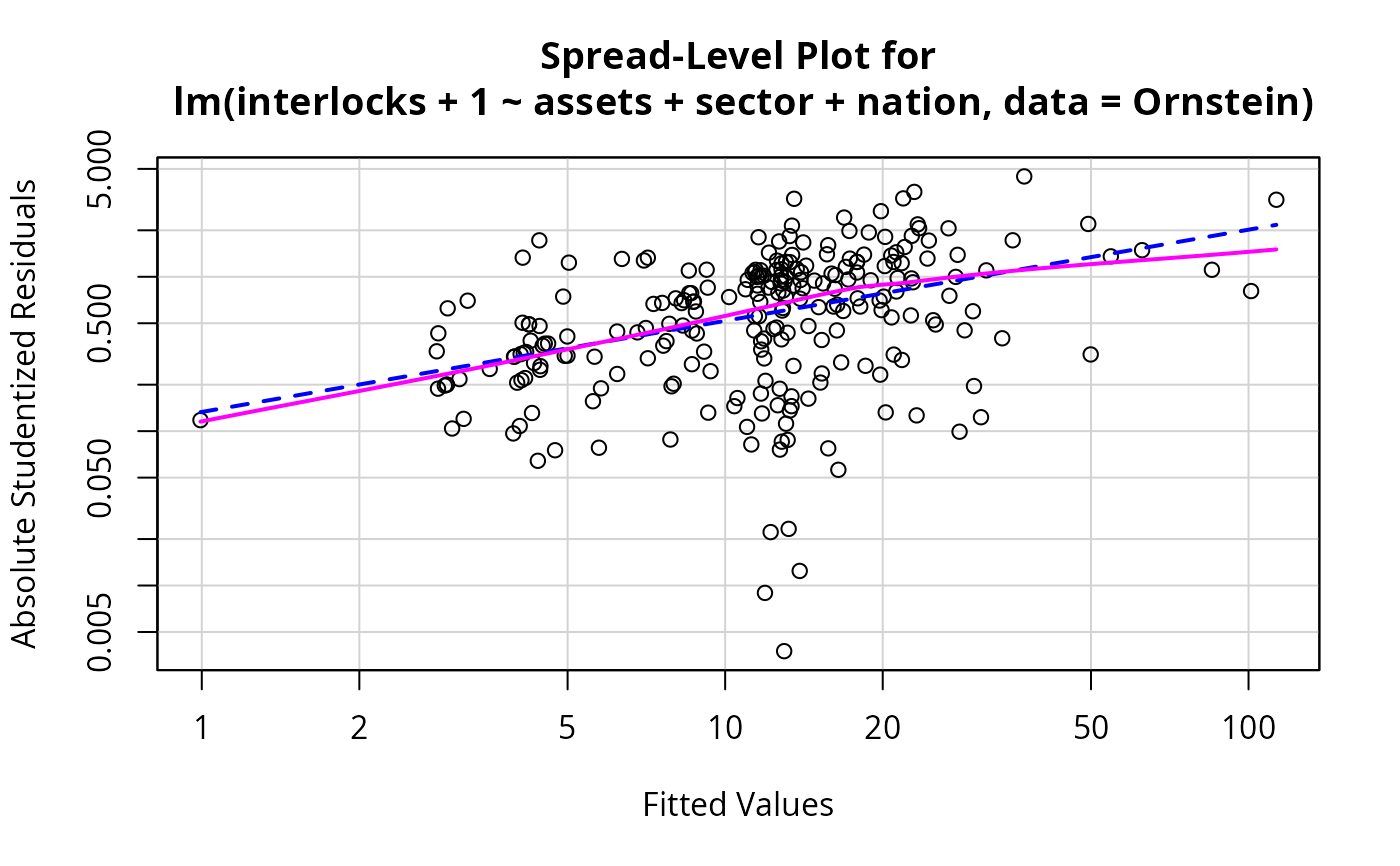#> Suggested power transformation:  0.4096738