Quantile-Comparison Plot
qqPlot.RdPlots empirical quantiles of a variable, or of studentized residuals from
a linear model, against theoretical quantiles of a comparison distribution. Includes
options not available in the qqnorm function.
Usage
qqPlot(x, ...)

qqp(...)

# Default S3 method
qqPlot(x, distribution="norm", groups, layout,
    ylim=range(x, na.rm=TRUE), ylab=deparse(substitute(x)),
    xlab=paste(distribution, "quantiles"), glab=deparse(substitute(groups)),
    main=NULL, las=par("las"),
    envelope=TRUE, col=carPalette()[1], col.lines=carPalette()[2],
    lwd=2, pch=1, cex=par("cex"),
    line=c("quartiles", "robust", "none"), id=TRUE, grid=TRUE, ...)

# S3 method for class 'formula'
qqPlot(formula, data, subset, id=TRUE, ylab, glab, ...)

# S3 method for class 'lm'
qqPlot(x, xlab=paste(distribution, "Quantiles"),
    ylab=paste("Studentized Residuals(",
                deparse(substitute(x)), ")", sep=""),
    main=NULL, distribution=c("t", "norm"),
    line=c("robust", "quartiles", "none"), las=par("las"),
    simulate=TRUE, envelope=TRUE,  reps=100,
    col=carPalette()[1], col.lines=carPalette()[2], lwd=2, pch=1, cex=par("cex"),
    id=TRUE, grid=TRUE, ...)
Arguments
- x
vector of numeric values or
lmobject.- distribution
root name of comparison distribution – e.g.,
"norm"for the normal distribution;tfor the t-distribution.- groups
an optional factor; if specified, a QQ plot will be drawn for
xwithin each level ofgroups.- layout
a 2-vector with the number of rows and columns for plotting by groups – for example
c(1, 3)for 1 row and 3 columns; if omitted, the number of rows and columns will be selected automatically; the specified number of rows and columns must be sufficient to accomodate the number of groups; ignored if there is no grouping factor.- formula
one-sided formula specifying a single variable to be plotted or a two-sided formula of the form
variable ~ factor, where a QQ plot will be drawn forvariablewithin each level offactor.- data
optional data frame within which to evaluage the formula.
- subset
optional subset expression to select cases to plot.
- ylim
limits for vertical axis; defaults to the range of
x. If plotting by groups, a common y-axis is used for all groups.- ylab
label for vertical (empirical quantiles) axis.
- xlab
label for horizontal (comparison quantiles) axis.
- glab
label for the grouping variable.
- main
label for plot.
- envelope
TRUE(the default),FALSE, a confidence level such as0.95, or a list specifying how to plot a point-wise confidence envelope (see Details).- las
if
0, ticks labels are drawn parallel to the axis; set to1for horizontal labels (seepar).- col
color for points; the default is the first entry in the current car palette (see
carPaletteandpar).- col.lines
color for lines; the default is the second entry in the current car palette.
- pch
plotting character for points; default is
1(a circle, seepar).- cex
factor for expanding the size of plotted symbols; the default is
1.- id
controls point identification; if
FALSE, no points are identified; can be a list of named arguments to theshowLabelsfunction;TRUEis equivalent tolist(method="y", n=2, cex=1, col=carPalette()[1], location="lr"), which identifies the 2 points with the 2 points with the most extreme verical values — studentized residuals for the"lm"method. Points labels are by default taken from the names of the variable being plotted is any, else case indices are used. Unlike most graphical functions in car, the default isid=TRUEto include point identification.- lwd
line width; default is
2(seepar).- line
"quartiles"to pass a line through the quartile-pairs, or"robust"for a robust-regression line; the latter uses therlmfunction in theMASSpackage. Specifyingline = "none"suppresses the line.- simulate
if
TRUEcalculate confidence envelope by parametric bootstrap; forlmobject only. The method is due to Atkinson (1985).- reps
integer; number of bootstrap replications for confidence envelope.
- ...
arguments such as
dfto be passed to the appropriate quantile function.- grid
If TRUE, the default, a light-gray background grid is put on the graph
Details
Draws theoretical quantile-comparison plots for variables and for studentized residuals from a linear model. A comparison line is drawn on the plot either through the quartiles of the two distributions, or by robust regression.
Any distribution for which quantile and
density functions exist in R (with prefixes q and d, respectively) may be used.
When plotting a vector, the confidence envelope is based on the SEs of the order statistics
of an independent random sample from the comparison distribution (see Fox, 2016).
Studentized residuals from linear models are plotted against the appropriate t-distribution with a point-wise
confidence envelope computed by default by a parametric bootstrap,
as described by Atkinson (1985).
The function qqp is an abbreviation for qqPlot.
The envelope argument can take a list with the following named elements; if an element is missing, then the default value is used:
levelconfidence level (default
0.95).styleone of
"filled"(the default),"lines", or"none".colcolor (default is the value of
col.lines).alphatransparency/opacity of a filled confidence envelope, a number between 0 and 1 (default
0.15).bordercontrols whether a border is drawn around a filled confidence envelope (default
TRUE).
Value
These functions return the labels of identified points, unless a grouping factor is employed,
in which case NULL is returned invisibly.
References
Fox, J. (2016) Applied Regression Analysis and Generalized Linear Models, Third Edition. Sage.
Fox, J. and Weisberg, S. (2019) An R Companion to Applied Regression, Third Edition, Sage.
Atkinson, A. C. (1985) Plots, Transformations, and Regression. Oxford.
Author
John Fox jfox@mcmaster.ca
Examples
x<-rchisq(100, df=2)
qqPlot(x)
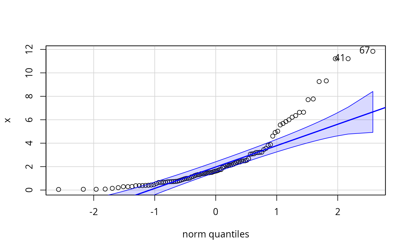 #> [1] 67 41
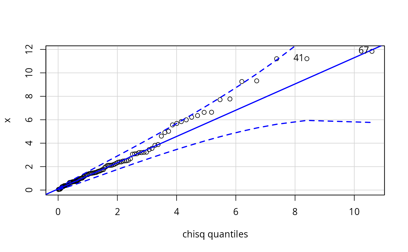
qqPlot(x, dist="chisq", df=2, envelope=list(style="lines"))
#> [1] 67 41
qqPlot(x, dist="chisq", df=2, envelope=list(style="lines"))
 #> [1] 67 41
qqPlot(~ income, data=Prestige, subset = type == "prof")
#> [1] 67 41
qqPlot(~ income, data=Prestige, subset = type == "prof")
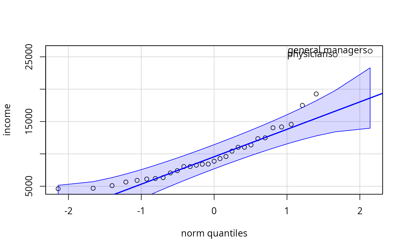 #> general.managers physicians
#> 2 24
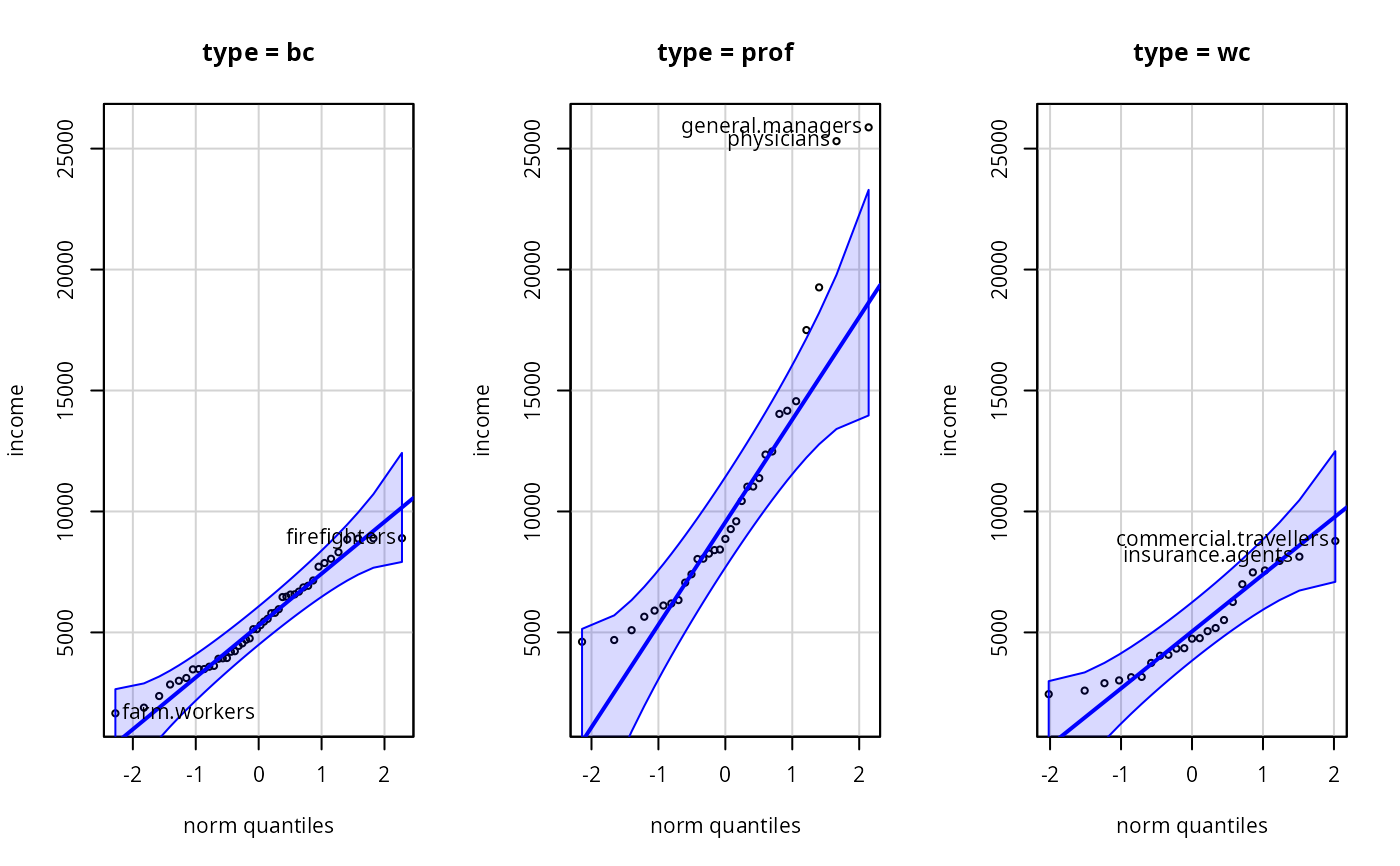
qqPlot(income ~ type, data=Prestige, layout=c(1, 3))
#> general.managers physicians
#> 2 24
qqPlot(income ~ type, data=Prestige, layout=c(1, 3))
 qqPlot(lm(prestige ~ income + education + type, data=Duncan),
envelope=.99)
qqPlot(lm(prestige ~ income + education + type, data=Duncan),
envelope=.99)
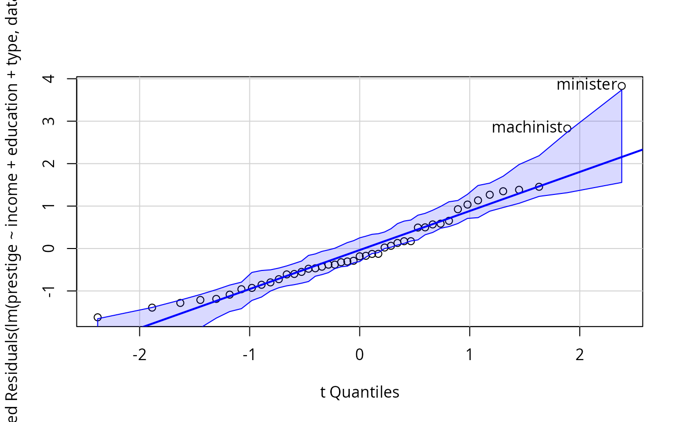 #> minister machinist
#> 6 28
#> minister machinist
#> 6 28