Marginal Model Plotting

For a regression object, draw a plot of the response on the vertical axis versus a linear combination \(u\) of regressors in the mean function on the horizontal axis. Added to the plot are a smooth for the graph, along with a smooth from the plot of the fitted values on \(u\). mmps is an alias for marginalModelPlots, and mmp is an alias for marginalModelPlot.

Usage

marginalModelPlots(...)

mmps(model, terms= ~ ., fitted=TRUE, layout=NULL, ask,
        main, groups, key=TRUE, ...)

marginalModelPlot(...)

mmp(model, ...)

# S3 method for class 'lm'
mmp(model, variable, sd = FALSE,
    xlab = deparse(substitute(variable)), 
    smooth=TRUE, key=TRUE, pch, groups=NULL, ...)

# Default S3 method
mmp(model, variable, sd = FALSE,
    xlab = deparse(substitute(variable)), ylab, smooth=TRUE,
    key=TRUE, pch, groups=NULL,
    col.line = carPalette()[c(2, 8)], col=carPalette()[1],
    id=FALSE, grid=TRUE, ...)

# S3 method for class 'glm'
mmp(model, variable, sd = FALSE,
    xlab = deparse(substitute(variable)), ylab,
    smooth=TRUE, key=TRUE, pch, groups=NULL,
    col.line = carPalette()[c(2, 8)], col=carPalette()[1],
    id=FALSE, grid=TRUE, ...)

Arguments

model: A regression object, usually of class either lm or glm, for which there is a predict method defined.
terms: A one-sided formula. A marginal model plot will be drawn for each term on the right-side of this formula that is not a factor. The default is ~ ., which specifies that all the terms in formula(object) will be used. If a conditioning argument is given, eg terms = ~. | a, then separate colors and smoothers are used for each unique non-missing value of a. See examples below.
fitted: If TRUE, the default, then a marginal model plot in the direction of the fitted values for a linear model or the linear predictor of a generalized linear model will be drawn.
layout: If set to a value like c(1, 1) or c(4, 3), the layout of the graph will have this many rows and columns. If not set, the program will select an appropriate layout. If the number of graphs exceed nine, you must select the layout yourself, or you will get a maximum of nine per page. If layout=NA, the function does not set the layout and the user can use the par function to control the layout, for example to have plots from two models in the same graphics window.
ask: If TRUE, ask before clearing the graph window to draw more plots.
main: Main title for the array of plots. Use main="" to suppress the title; if missing, a title will be supplied.
...: Additional arguments passed from mmps to mmp and then to plot. Users should generally use mmps, or equivalently marginalModelPlots.
variable: The quantity to be plotted on the horizontal axis. If this argument is missing, the horizontal variable is the linear predictor, returned by predict(object) for models of class lm, with default label "Fitted values", or returned by predict(object, type="link") for models of class glm, with default label "Linear predictor". It can be any other vector of length equal to the number of observations in the object. Thus the mmp function can be used to get a marginal model plot versus any regressor or predictor while the mmps function can be used only to get marginal model plots for the first-order regressors in the formula. In particular, terms defined by a spline basis are skipped by mmps, but you can use mmp to get the plot for the variable used to define the splines.
sd: If TRUE, display sd smooths. For a binomial regression with all sample sizes equal to one, this argument is ignored as the SD bounds don't make any sense.
xlab: label for horizontal axis.
ylab: label for vertical axis, defaults to name of response.
smooth: specifies the smoother to be used along with its arguments; if FALSE, no smoother is shown; can be a list giving the smoother function and its named arguments; TRUE, the default, is equivalent to list(smoother=loessLine, span=2/3) for linear models and list(smoother=gamLine, k=3) for generalized linear models. See ScatterplotSmoothers for the smoothers supplied by the car package and their arguments; the spread argument is not supported for marginal model plots.
groups: The name of a vector that specifies a grouping variable for separate colors/smoothers. This can also be specified as a conditioning argument on the terms argument.
key: If TRUE, include a key at the top of the plot, if FALSE omit the key. If grouping is present, the key is only printed for the upper-left plot.
id: controls point identification; if FALSE (the default), no points are identified; can be a list of named arguments to the showLabels function; TRUE is equivalent to list(method="y", n=2, cex=1, col=carPalette()[1], location="lr"), which identifies the 2 points with the most unusual response (Y) values.
pch: plotting character to use if no grouping is present.
col.line: colors for data and model smooth, respectively. The default is to use carPalette, carPalette()[c(2, 8)], blue and red.
col: color(s) for the plotted points.
grid: If TRUE, the default, a light-gray background grid is put on the graph

Details

mmp and marginalModelPlot draw one marginal model plot against whatever is specified as the horizontal axis. mmps and marginalModelPlots draws marginal model plots versus each of the terms in the terms argument and versus fitted values. mmps skips factors and interactions if they are specified in the terms argument. Terms based on polynomials or on splines (or potentially any term that is represented by a matrix of regressors) will be used to form a marginal model plot by returning a linear combination of the terms. For example, if you specify terms = ~ X1 + poly(X2, 3) and poly(X2, 3) was part of the original model formula, the horizontal axis of the marginal model plot for X2 will be the value of predict(model, type="terms")[, "poly(X2, 3)"]). If the predict method for the model you are using doesn't support type="terms", then the polynomial/spline term is skipped. Adding a conditioning variable, e.g., terms = ~ a + b | c, will produce marginal model plots for a and b with different colors and smoothers for each unique non-missing value of c.

For linear models, the default smoother is loess. For generalized linear models, the default smoother uses gamLine, fitting a generalized additive model with the same family, link and weights as the fit of the model. SD smooths are not computed for for generalized linear models.

For generalized linear models the default number of elements in the spline basis is k=3; this is done to allow fitting for predictors with just a few support points. If you have many support points you may wish to set k to a higher number, or k=-1 for the default used by gam.

Value

Used for its side effect of producing plots.

References

Cook, R. D., & Weisberg, S. (1997). Graphics for assessing the adequacy of regression models. Journal of the American Statistical Association, 92(438), 490-499.

Fox, J. and Weisberg, S. (2019) An R Companion to Applied Regression, Third Edition. Sage.

Weisberg, S. (2005) Applied Linear Regression, Third Edition, Wiley, Section 8.4.

Author

Sanford Weisberg, sandy@umn.edu

Examples

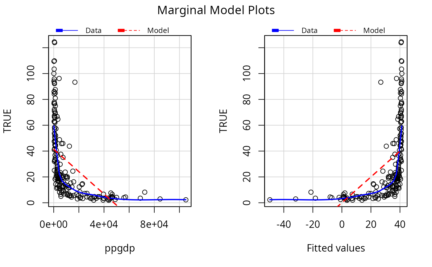
c1 <- lm(infantMortality ~ ppgdp, UN)
mmps(c1)

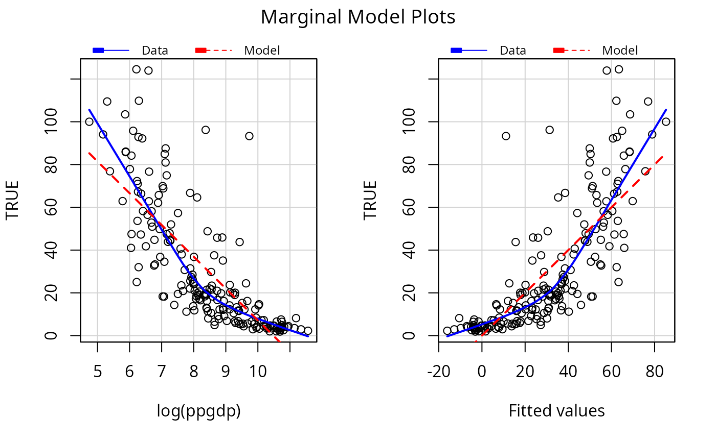
c2 <- update(c1, ~ log(ppgdp))
mmps(c2)

# include SD lines
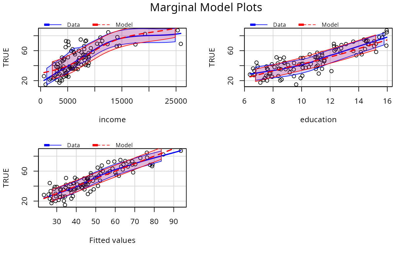
p1 <- lm(prestige ~ income + education, Prestige)
mmps(p1, sd=TRUE)

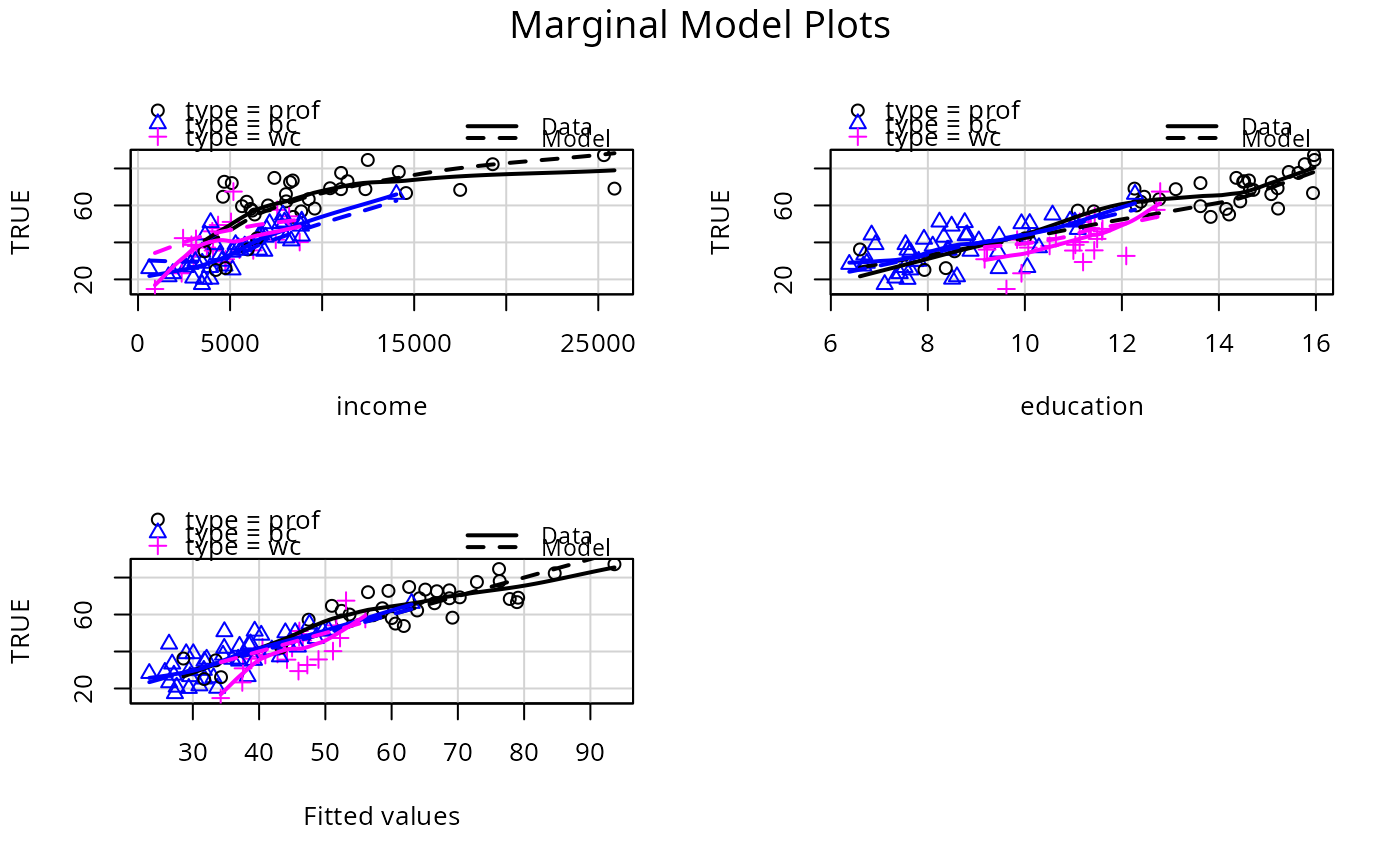
# condition on type:
mmps(p1, ~. | type)

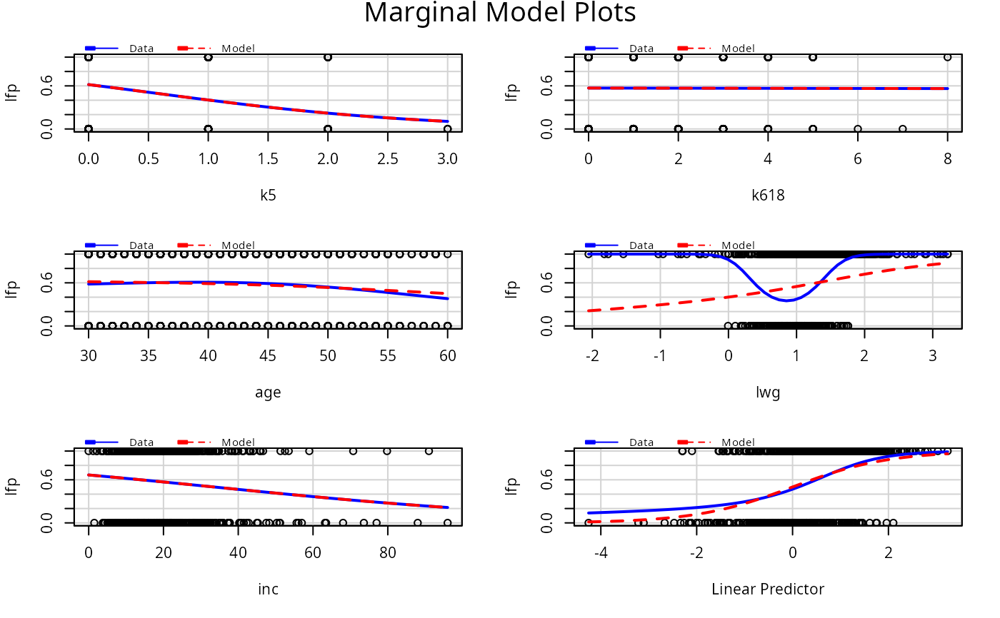
# logisitic regression example
# smoothers return warning messages.
# fit a separate smoother and color for each type of occupation.
m1 <- glm(lfp ~ ., family=binomial, data=Mroz)
mmps(m1)

#> Warning: Interactions and/or factors skipped