Regression Influence Plot

This function creates a “bubble” plot of Studentized residuals versus hat values, with the areas of the circles representing the observations proportional to the value Cook's distance. Vertical reference lines are drawn at twice and three times the average hat value, horizontal reference lines at -2, 0, and 2 on the Studentized-residual scale.

Usage

influencePlot(model, ...)

# S3 method for class 'lm'
influencePlot(model, scale=10,  
 xlab="Hat-Values", ylab="Studentized Residuals", id=TRUE, 
 fill=TRUE, fill.col=carPalette()[2], fill.alpha=0.5, ...)

# S3 method for class 'lmerMod'
influencePlot(model, ...)

Arguments

model: a linear, generalized-linear, or linear mixed model; the "lmerMod" method calls the "lm" method and can take the same arguments.
scale: a factor to adjust the size of the circles.
xlab, ylab: axis labels.
id: settings for labelling points; see link{showLabels} for details. To omit point labelling, set id=FALSE; the default, id=TRUE is equivalent to id=list(method="noteworthy", n=2, cex=1, col=carPalette()[1], location="lr"). The default method="noteworthy" is used only in this function and indicates setting labels for points with large Studentized residuals, hat-values or Cook's distances. Set id=list(method="identify") for interactive point identification.
fill: if TRUE (the default) fill the circles, with the opacity of the filled color proportional to Cook's D, using the alpha function in the scales package to compute the opacity of the fill.
fill.col: color to use for the filled points, taken by default from the second element of the carPalette color palette.
fill.alpha: the maximum alpha (opacity) of the points.
...: arguments to pass to the plot and points functions.

Value

If points are identified, returns a data frame with the hat values, Studentized residuals and Cook's distance of the identified points. If no points are identified, nothing is returned. This function is primarily used for its side-effect of drawing a plot.

References

Fox, J. (2016) Applied Regression Analysis and Generalized Linear Models, Third Edition. Sage.

Fox, J. and Weisberg, S. (2019) An R Companion to Applied Regression, Third Edition, Sage.

Author

John Fox jfox@mcmaster.ca, minor changes by S. Weisberg sandy@umn.edu and a contribution from Michael Friendly

Examples

influencePlot(lm(prestige ~ income + education, data=Duncan))

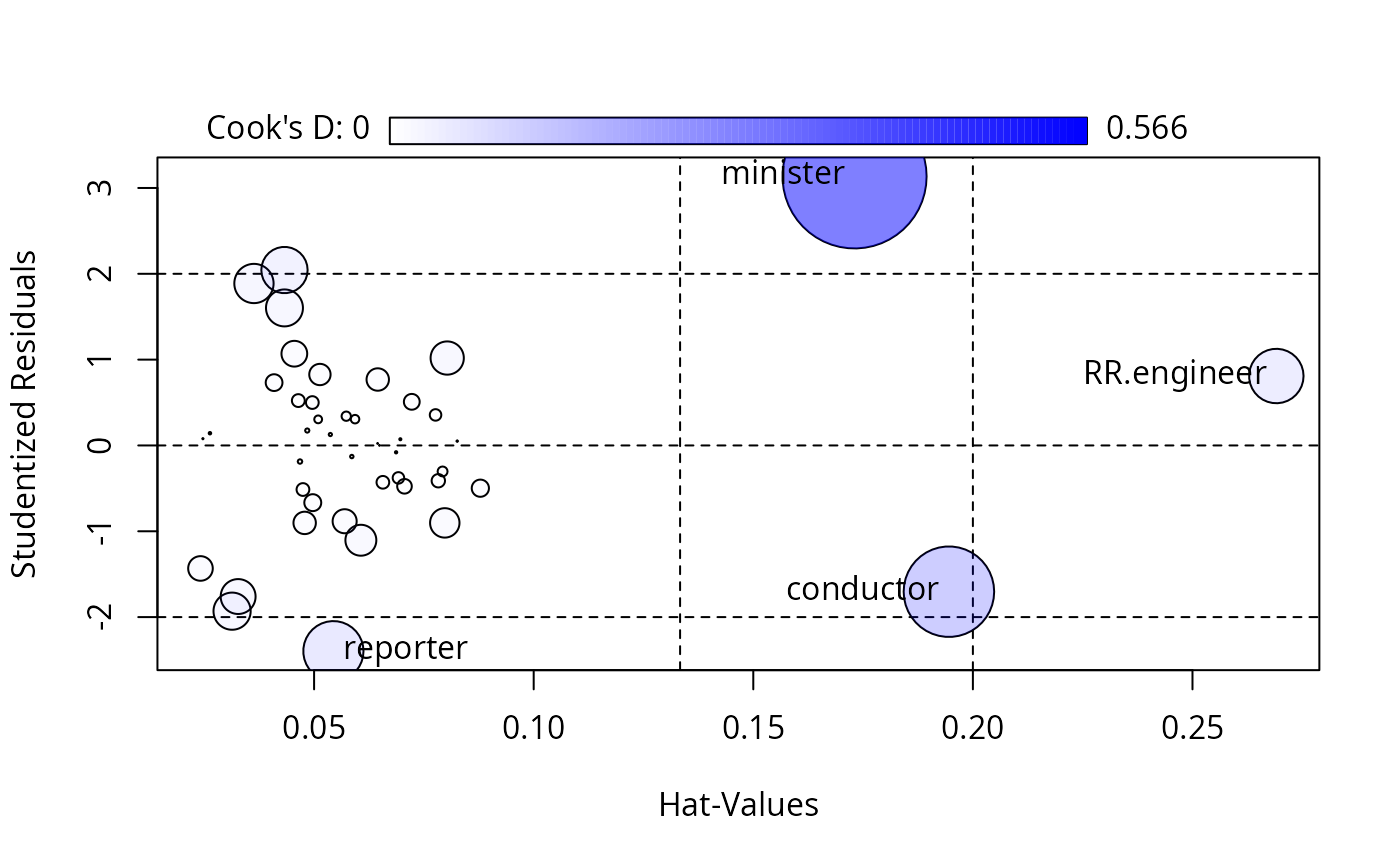#>                StudRes        Hat      CookD
#> minister     3.1345186 0.17305816 0.56637974
#> reporter    -2.3970224 0.05439356 0.09898456
#> conductor   -1.7040324 0.19454165 0.22364122
#> RR.engineer  0.8089221 0.26908963 0.08096807
if (FALSE)  # requires user interaction to identify points
influencePlot(lm(prestige ~ income + education, data=Duncan), 
    id=list(method="identify"))
 # \dontrun{}