Axes for Transformed Variables
TransformationAxes.RdThese functions produce axes for the original scale of
transformed variables. Typically these would appear as additional
axes to the right or
at the top of the plot, but if the plot is produced with
axes=FALSE, then these functions could be used for axes below or to
the left of the plot as well.
Usage
basicPowerAxis(power, base=exp(1),
    side=c("right", "above", "left", "below"),
    at, start=0, lead.digits=1, n.ticks, grid=FALSE, grid.col=gray(0.50),
    grid.lty=2,
    axis.title="Untransformed Data", cex=1, las=par("las"))

bcPowerAxis(power, side=c("right", "above", "left", "below"),
    at, start=0, lead.digits=1, n.ticks, grid=FALSE, grid.col=gray(0.50),
    grid.lty=2,
    axis.title="Untransformed Data", cex=1, las=par("las"))

bcnPowerAxis(power, shift, side=c("right", "above", "left", "below"),
    at, start=0, lead.digits=1, n.ticks, grid=FALSE, grid.col=gray(0.50),
    grid.lty=2,
    axis.title="Untransformed Data", cex=1, las=par("las"))

yjPowerAxis(power, side=c("right", "above", "left", "below"),
  at, lead.digits=1, n.ticks, grid=FALSE, grid.col=gray(0.50),
  grid.lty=2,
  axis.title="Untransformed Data", cex=1, las=par("las"))

probabilityAxis(scale=c("logit", "probit"),
  side=c("right", "above", "left", "below"),
  at, lead.digits=1, grid=FALSE, grid.lty=2, grid.col=gray(0.50),
    axis.title = "Probability", interval = 0.1, cex = 1, las=par("las"))
Arguments
- power
power for Box-Cox, Box-Cox with negatives, Yeo-Johnson, or simple power transformation.
- shift
the shift (gamma) parameter for the Box-Cox with negatives family.
- scale
transformation used for probabilities,
"logit"(the default) or"probit".- side
side at which the axis is to be drawn; numeric codes are also permitted:
side = 1for the bottom of the plot,side=2for the left side,side = 3for the top,side = 4for the right side.- at
numeric vector giving location of tick marks on original scale; if missing, the function will try to pick nice locations for the ticks.
- start
if a start was added to a variable (e.g., to make all data values positive), it can now be subtracted from the tick labels.
- lead.digits
number of leading digits for determining `nice' numbers for tick labels (default is
1.- n.ticks
number of tick marks; if missing, same as corresponding transformed axis.
- grid
if
TRUEgrid lines for the axis will be drawn.- grid.col
color of grid lines.
- grid.lty
line type for grid lines.
- axis.title
title for axis.
- cex
relative character expansion for axis label.
- las
if
0, ticks labels are drawn parallel to the axis; set to1for horizontal labels (seepar).- base
base of log transformation for
power.axiswhenpower = 0.- interval
desired interval between tick marks on the probability scale.
Details
The transformations corresponding to the three functions are as follows:
basicPowerAxis:Simple power transformation, \(x^{\prime }=x^{p}\) for \(p\neq 0\) and \(x^{\prime }=\log x\) for \(p=0\).
bcPowerAxis:Box-Cox power transformation, \(x^{\prime }=(x^{\lambda }-1)/\lambda\) for \(\lambda \neq 0\) and \(x^{\prime }=\log x\) for \(\lambda =0\).
bcnPowerAxis:Box-Cox with negatives power transformation, the Box-Cox power transformation of \(z = .5 * (y + (y^2 + \gamma^2)^{1/2})\), where \(\gamma\) is strictly positive if \(y\) includes negative values and non-negative otherwise. The value of \(z\) is always positive.
yjPowerAxis:Yeo-Johnson power transformation, for non-negative \(x\), the Box-Cox transformation of \(x + 1\); for negative \(x\), the Box-Cox transformation of \(|x| + 1\) with power \(2 - p\).
probabilityAxis:logit or probit transformation, logit \(=\log [p/(1-p)]\), or probit \(=\Phi^{-1}(p)\), where \(\Phi^{-1}\) is the standard-normal quantile function.
These functions will try to place tick marks at reasonable locations, but
producing a good-looking graph sometimes requires some fiddling with the
at argument.
Author
John Fox jfox@mcmaster.ca
References
Fox, J. and Weisberg, S. (2019) An R Companion to Applied Regression, Third Edition, Sage.
Examples
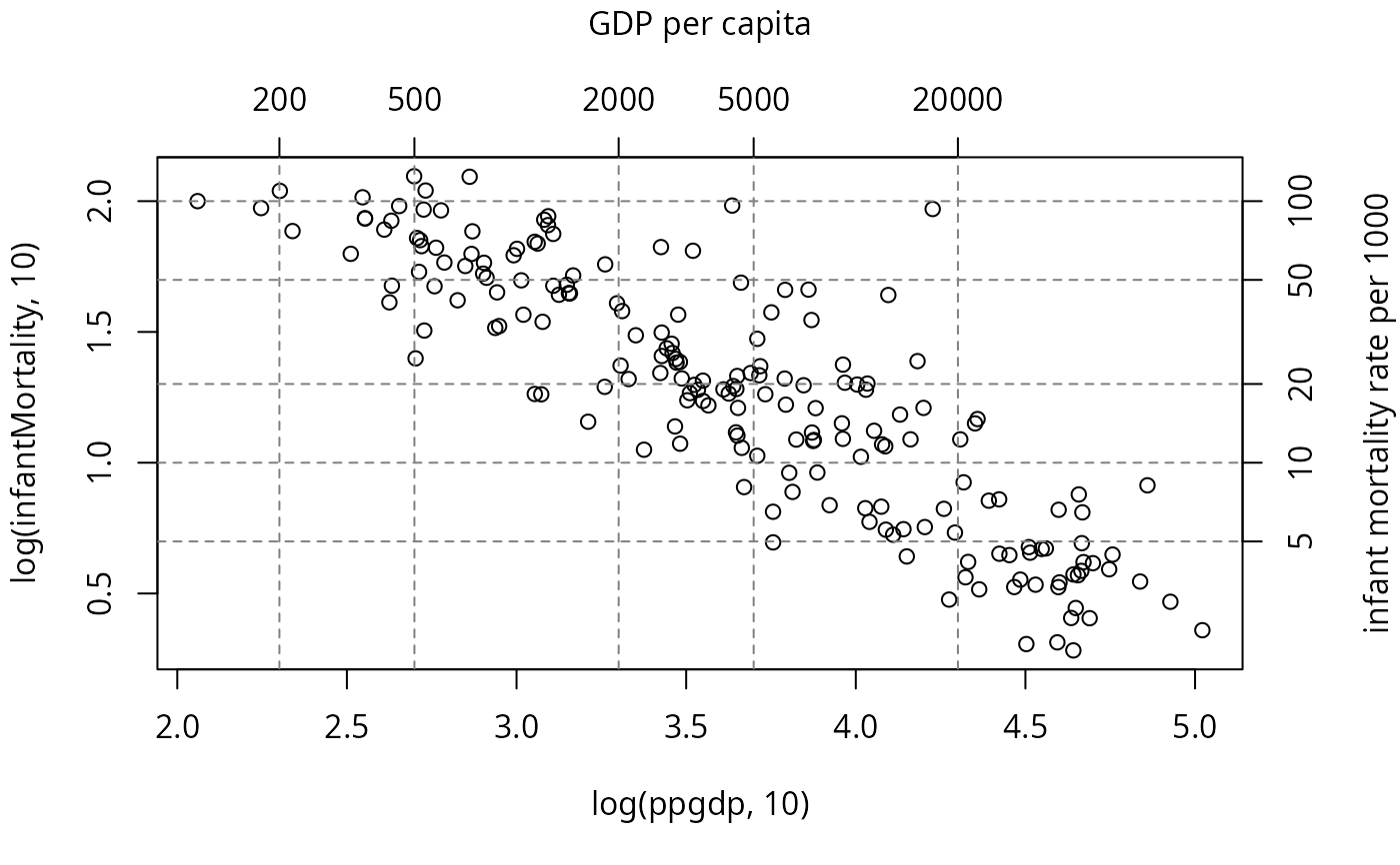
UN <- na.omit(UN)
par(mar=c(5, 4, 4, 4) + 0.1) # leave space on right
with(UN, plot(log(ppgdp, 10), log(infantMortality, 10)))
basicPowerAxis(0, base=10, side="above",
at=c(50, 200, 500, 2000, 5000, 20000), grid=TRUE,
axis.title="GDP per capita")
basicPowerAxis(0, base=10, side="right",
at=c(5, 10, 20, 50, 100), grid=TRUE,
axis.title="infant mortality rate per 1000")
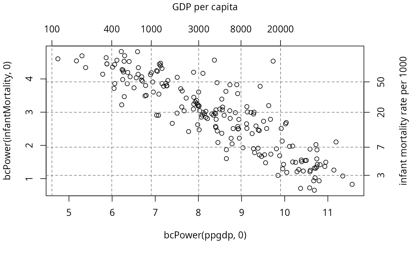
 with(UN, plot(bcPower(ppgdp, 0), bcPower(infantMortality, 0)))
bcPowerAxis(0, side="above",
grid=TRUE, axis.title="GDP per capita")
bcPowerAxis(0, side="right",
grid=TRUE, axis.title="infant mortality rate per 1000")
with(UN, plot(bcPower(ppgdp, 0), bcPower(infantMortality, 0)))
bcPowerAxis(0, side="above",
grid=TRUE, axis.title="GDP per capita")
bcPowerAxis(0, side="right",
grid=TRUE, axis.title="infant mortality rate per 1000")
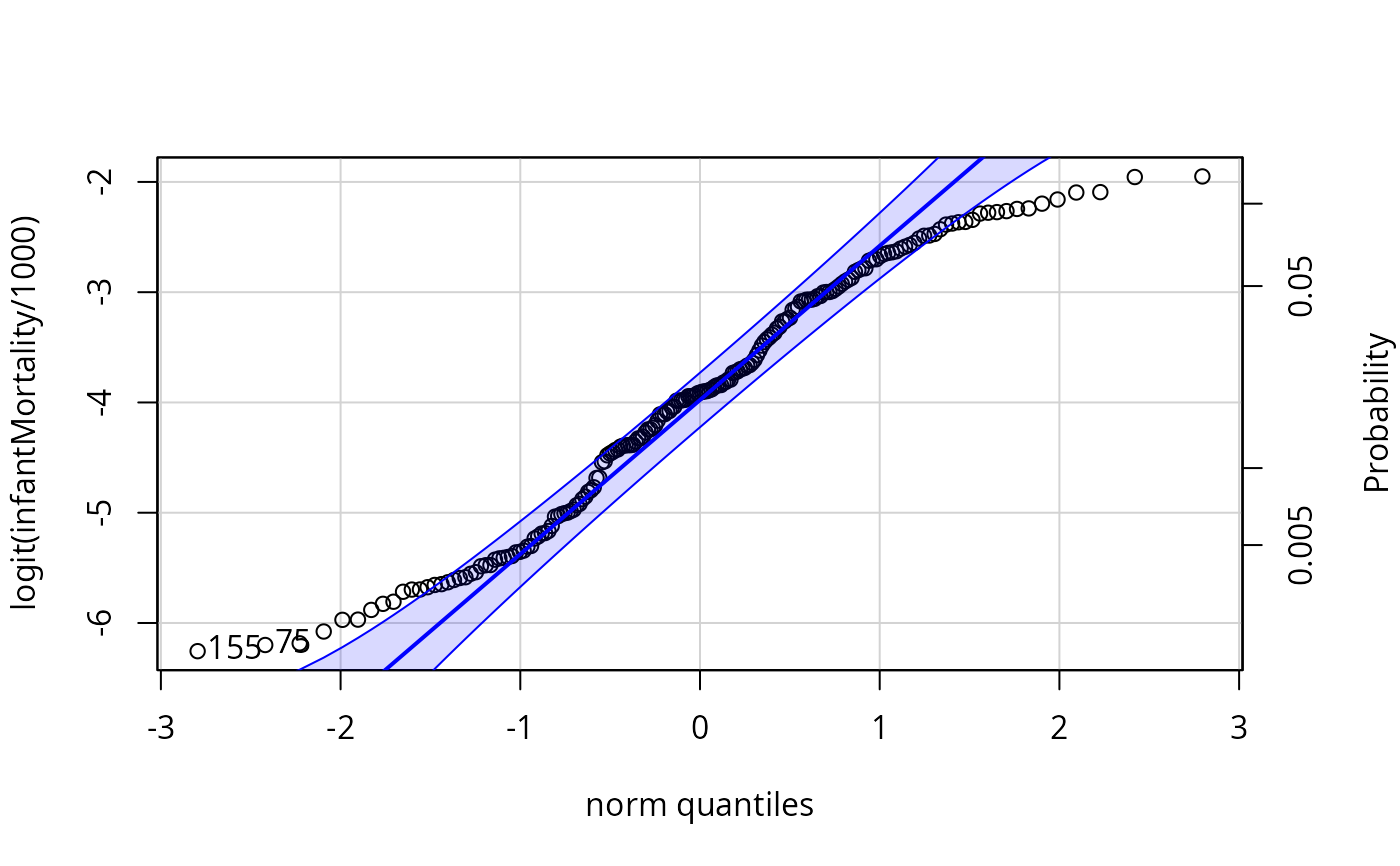
 with(UN, qqPlot(logit(infantMortality/1000)))
#> [1] 155 75
probabilityAxis()
with(UN, qqPlot(logit(infantMortality/1000)))
#> [1] 155 75
probabilityAxis()
 with(UN, qqPlot(qnorm(infantMortality/1000)))
#> [1] 1 33
probabilityAxis(at=c(.005, .01, .02, .04, .08, .16), scale="probit")
with(UN, qqPlot(qnorm(infantMortality/1000)))
#> [1] 1 33
probabilityAxis(at=c(.005, .01, .02, .04, .08, .16), scale="probit")
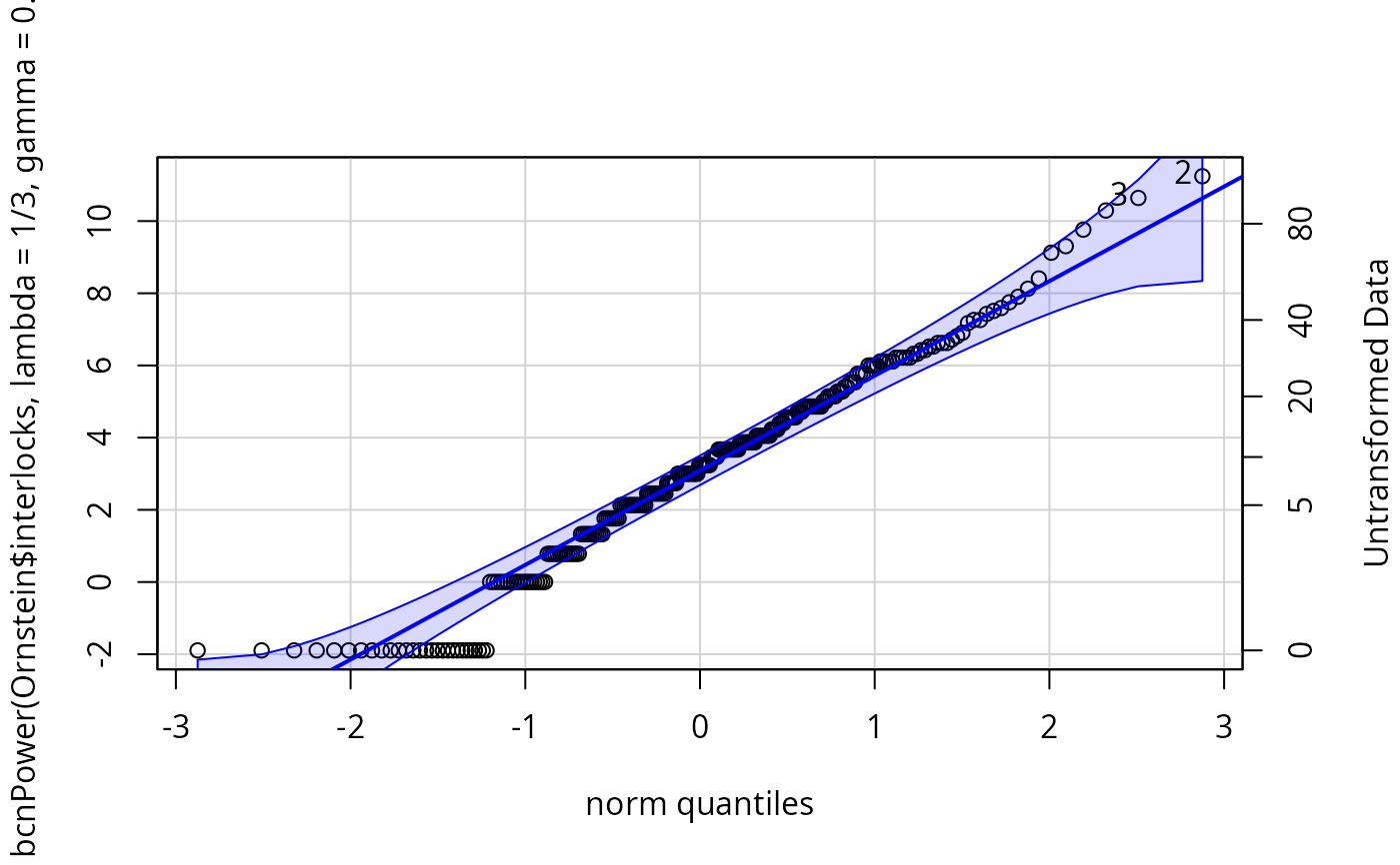
 qqPlot(bcnPower(Ornstein$interlocks, lambda=1/3, gamma=0.1))
#> [1] 2 3
bcnPowerAxis(1/3, 0.1, at=c(o=0, 5, 10, 20, 40, 80))
qqPlot(bcnPower(Ornstein$interlocks, lambda=1/3, gamma=0.1))
#> [1] 2 3
bcnPowerAxis(1/3, 0.1, at=c(o=0, 5, 10, 20, 40, 80))