Before we measure performance of the main functionality of the
package, note that something simple as ‘(a:b)[-i]’ can and has been
accelerated in this package:
a <- 1L
b <- 1e7L
i <- sample(a:b, 1e3)
x <- c(
  R = median(microbenchmark((a:b)[-i], times=times)$time),
  bit = median(microbenchmark(bit_rangediff(c(a, b), i), times=times)$time),
  merge = median(microbenchmark(merge_rangediff(c(a, b), bit_sort(i)), times=times)$time)
)
knitr::kable(as.data.frame(as.list(x / x["R"] * 100)), caption="% of time relative to R", digits=1)
% of time relative to R
| 100 |
28.7 |
24.6 |
The vignette is compiled with the following performance settings: 5
replications with domain size small 1000 and big 10^{6}, sample size
small 1000 and big 10^{6}.
Boolean data types
“A designer knows he has achieved perfection not when there is
nothing left to add, but when there is nothing left to take away.” “Il
semble que la perfection soit atteinte non quand il n’y a plus rien à
ajouter, mais quand il n’y a plus rien à retrancher” (Antoine de
St. Exupery, Terre des Hommes (Gallimard, 1939), p. 60.)
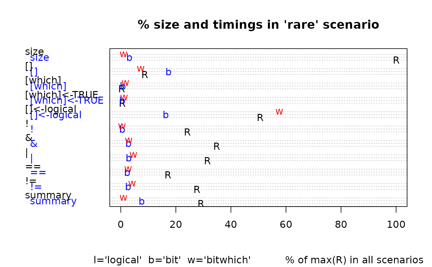
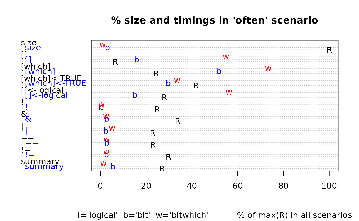
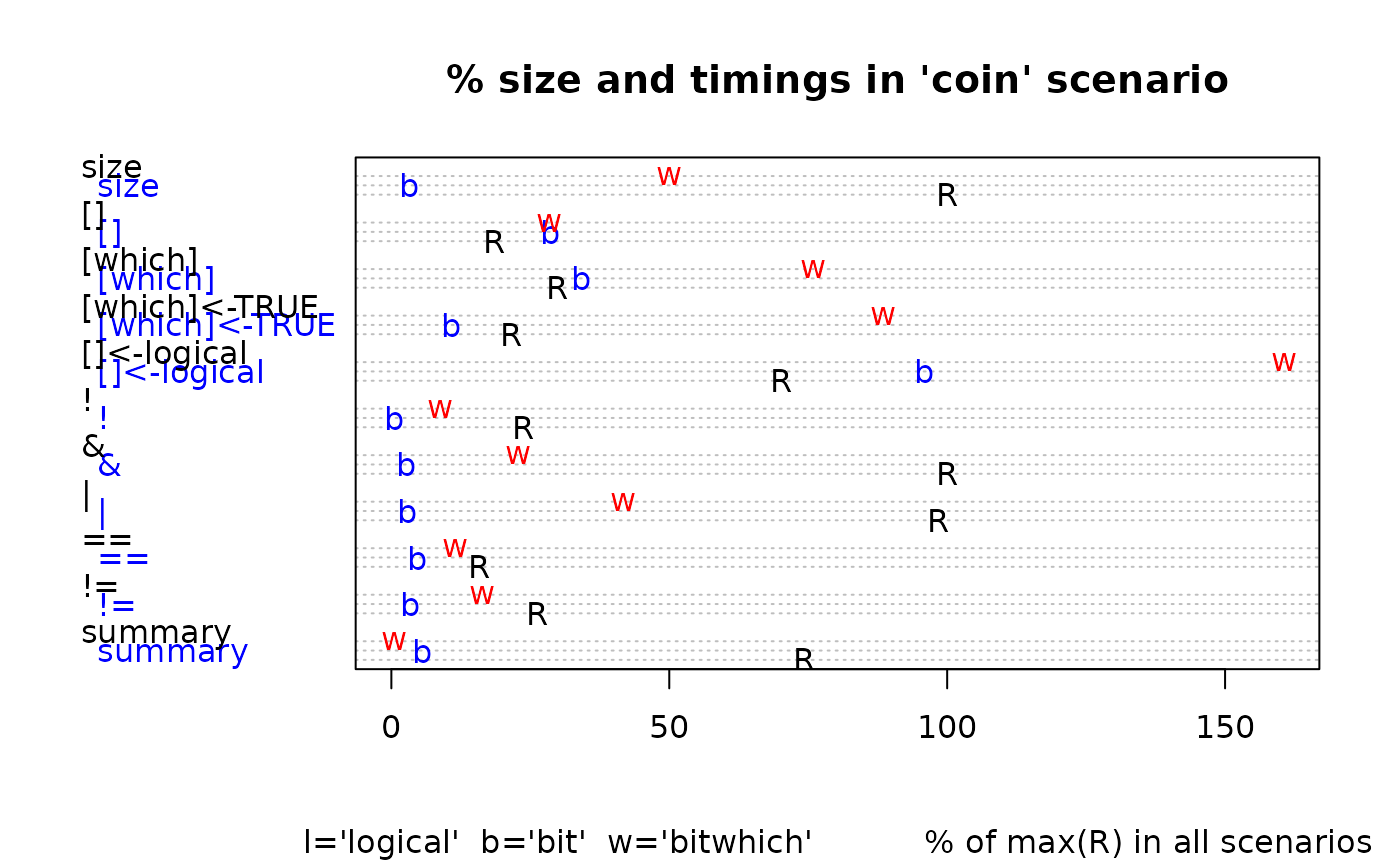
We compare memory consumption (n=1e+06) and runtime (median of 5
replications) of the different booltypes for the following
filter scenarios:
knitr::kable(
  data.frame(
    coin="random 50%",
    often="random 99%",
    rare="random 1%",
    chunk="contiguous chunk of 5%"
  ),
  caption="selection characteristic"
)
selection characteristic
| random 50% |
random 99% |
random 1% |
contiguous chunk of 5% |
# nolint end: strings_as_factors_linter.
There are substantial savings in skewed filter situations:
Even in non-skewed situations the new booltypes are competitive:
Detailed tables follow.
% memory consumption of filter
% bytes of logical
| logical |
100.0 |
100.0 |
100.0 |
100.0 |
| bit |
3.2 |
3.2 |
3.2 |
3.2 |
| bitwhich |
50.0 |
1.0 |
1.0 |
5.0 |
| which |
50.0 |
99.0 |
1.0 |
5.0 |
| ri |
NA |
NA |
NA |
0.0 |
% time of logical
| logical |
18.5 |
6.4 |
8.7 |
NA |
| bit |
28.5 |
15.9 |
17.4 |
NA |
| bitwhich |
28.4 |
54.9 |
7.3 |
NA |
| which |
NA |
NA |
NA |
NA |
| ri |
NA |
NA |
NA |
NA |
% time assigning
% time of logical
| logical |
70.1 |
28.0 |
50.6 |
NA |
| bit |
95.8 |
15.1 |
16.3 |
NA |
| bitwhich |
160.5 |
56.2 |
57.6 |
NA |
| which |
NA |
NA |
NA |
NA |
| ri |
NA |
NA |
NA |
NA |
% time subscripting with ‘which’
% time of logical
| logical |
29.8 |
24.4 |
0.3 |
NA |
| bit |
34.1 |
51.8 |
0.8 |
NA |
| bitwhich |
75.9 |
73.4 |
1.7 |
NA |
| which |
NA |
NA |
NA |
NA |
| ri |
NA |
NA |
NA |
NA |
% time assigning with ‘which’
% time of logical
| logical |
21.5 |
41.7 |
0.5 |
NA |
| bit |
10.8 |
29.7 |
0.5 |
NA |
| bitwhich |
88.5 |
33.6 |
1.2 |
NA |
| which |
NA |
NA |
NA |
NA |
| ri |
NA |
NA |
NA |
NA |
% time Boolean NOT
% time for Boolean NOT
| logical |
23.8 |
24.9 |
24.1 |
15.7 |
| bit |
0.5 |
0.5 |
0.5 |
0.5 |
| bitwhich |
8.8 |
0.5 |
0.5 |
1.0 |
| which |
NA |
NA |
NA |
NA |
| ri |
NA |
NA |
NA |
NA |
% time Boolean AND
% time for Boolean &
| logical |
100.0 |
33.9 |
34.8 |
12.6 |
| bit |
2.6 |
2.8 |
2.8 |
2.5 |
| bitwhich |
22.9 |
2.6 |
2.8 |
5.9 |
| which |
NA |
NA |
NA |
NA |
| ri |
NA |
NA |
NA |
NA |
% time Boolean OR
% time for Boolean |
| logical |
98.4 |
22.8 |
31.5 |
16.4 |
| bit |
2.9 |
2.5 |
2.9 |
4.9 |
| bitwhich |
41.6 |
5.1 |
4.5 |
4.5 |
| which |
NA |
NA |
NA |
NA |
| ri |
NA |
NA |
NA |
NA |
% time Boolean EQUALITY
% time for Boolean ==
| logical |
15.9 |
23.0 |
17.1 |
16.8 |
| bit |
4.7 |
2.9 |
2.4 |
3.1 |
| bitwhich |
11.5 |
2.7 |
2.7 |
3.5 |
| which |
NA |
NA |
NA |
NA |
| ri |
NA |
NA |
NA |
NA |
% time Boolean XOR
% time for Boolean !=
| logical |
26.3 |
29.8 |
27.7 |
17.6 |
| bit |
3.4 |
2.6 |
2.6 |
2.6 |
| bitwhich |
16.4 |
2.6 |
4.1 |
3.0 |
| which |
NA |
NA |
NA |
NA |
| ri |
NA |
NA |
NA |
NA |
% time Boolean SUMMARY
% time for Boolean summary
| logical |
74.3 |
26.8 |
| bit |
5.6 |
5.4 |
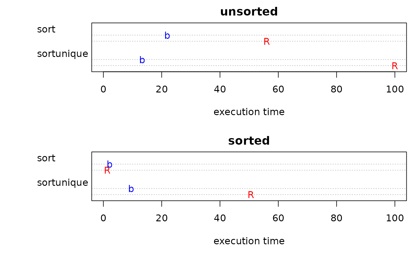
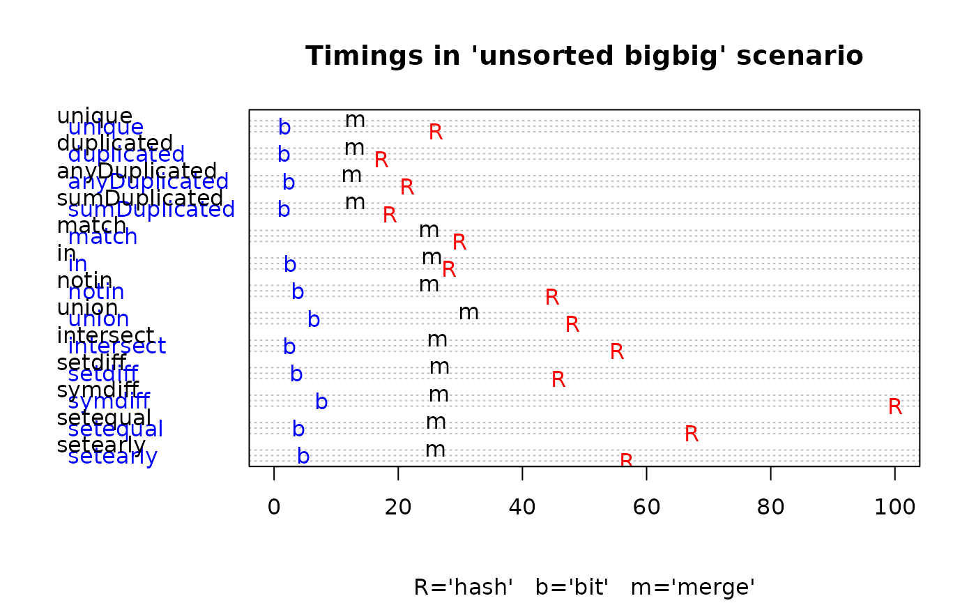
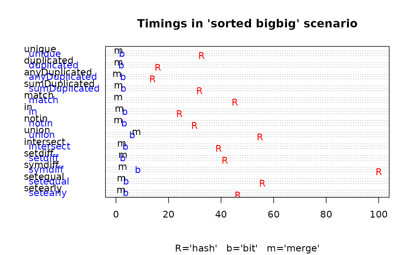
Fast methods for integer set operations
“The space-efficient structure of bitmaps dramatically reduced the
run time of sorting” (Jon Bently, Programming Pearls, Cracking the
oyster, p. 7)
% time for sorting
sorted data relative to R’s sort
| sort |
116.4 |
156.2 |
| sortunique |
53.9 |
18.8 |
unsorted data relative to R’s sort
| sort |
60.3 |
39.2 |
| sortunique |
36.2 |
13.3 |
% time for unique
sorted data relative to R
| bit |
88.9 |
6.8 |
| merge |
21.3 |
3.1 |
| sort |
0.0 |
0.0 |
unsorted data relative to R
| bit |
137.2 |
6.6 |
| merge |
263.5 |
50.1 |
| sort |
237.3 |
46.6 |
% time for duplicated
sorted data relative to R
| bit |
245.3 |
12.4 |
| merge |
40.4 |
5.7 |
| sort |
0.0 |
0.0 |
unsorted data relative to R
| bit |
246.2 |
9.4 |
| merge |
194.9 |
74.7 |
| sort |
172.1 |
69.9 |
% time for anyDuplicated
sorted data relative to R
| bit |
196.4 |
19.3 |
| merge |
36.7 |
2.9 |
| sort |
0.0 |
0.0 |
unsorted data relative to R
| bit |
229.3 |
10.8 |
| merge |
346.1 |
58.4 |
| sort |
309.0 |
56.6 |
% time for sumDuplicated
sorted data relative to R
| bit |
98.6 |
8.9 |
| merge |
19.9 |
3.2 |
| sort |
0.0 |
0.0 |
unsorted data relative to R
| bit |
54.2 |
8.7 |
| merge |
79.1 |
70.2 |
| sort |
69.6 |
65.2 |
% time for match
sorted data relative to R
| bit |
NA |
NA |
NA |
NA |
| merge |
27 |
0 |
6.4 |
1.8 |
| sort |
0 |
0 |
0.0 |
0.0 |
unsorted data relative to R
| bit |
NA |
NA |
NA |
NA |
| merge |
480.7 |
61.2 |
87.4 |
83.8 |
| sort |
451.3 |
61.2 |
84.8 |
81.3 |
% time for in
sorted data relative to R
| bit |
183.9 |
5.4 |
7.8 |
14.0 |
| merge |
25.2 |
0.0 |
11.3 |
5.3 |
| sort |
0.0 |
0.0 |
0.0 |
0.0 |
unsorted data relative to R
| bit |
184.3 |
5.7 |
4.5 |
9.2 |
| merge |
471.6 |
77.3 |
94.0 |
90.2 |
| sort |
443.2 |
77.3 |
88.4 |
86.0 |
% time for notin
sorted data relative to R
| bit |
210.1 |
3.8 |
10.6 |
10.6 |
| merge |
20.3 |
0.0 |
5.2 |
2.8 |
| sort |
0.0 |
0.0 |
0.0 |
0.0 |
unsorted data relative to R
| bit |
224.3 |
4.5 |
3.8 |
8.6 |
| merge |
380.3 |
56.1 |
80.8 |
55.8 |
| sort |
346.8 |
56.1 |
77.8 |
54.1 |
% time for union
sorted data relative to R
| bit |
77.2 |
22.7 |
23.4 |
11.3 |
| merge |
55.5 |
14.4 |
21.1 |
14.2 |
| sort |
0.0 |
0.0 |
0.0 |
0.0 |
unsorted data relative to R
| bit |
100.4 |
27.0 |
34.3 |
13.3 |
| merge |
349.1 |
68.2 |
89.9 |
65.4 |
| sort |
247.5 |
51.6 |
66.9 |
50.4 |
% time for intersect
sorted data relative to R
| bit |
38.4 |
7.4 |
3 |
9.2 |
| merge |
20.9 |
0.0 |
0 |
5.7 |
| sort |
0.0 |
0.0 |
0 |
0.0 |
unsorted data relative to R
| bit |
56.6 |
7.1 |
2.6 |
4.5 |
| merge |
192.6 |
60.4 |
35.2 |
47.5 |
| sort |
159.8 |
60.4 |
35.2 |
43.8 |
% time for setdiff
sorted data relative to R
| bit |
59.3 |
3.1 |
21.2 |
6.2 |
| merge |
16.5 |
0.0 |
15.5 |
6.4 |
| sort |
0.0 |
0.0 |
0.0 |
0.0 |
unsorted data relative to R
| bit |
74.1 |
3.4 |
15.6 |
7.8 |
| merge |
208.2 |
52.9 |
40.0 |
58.2 |
| sort |
183.1 |
52.9 |
30.7 |
52.9 |
% time for symdiff
sorted data relative to R
| bit |
31.9 |
9.9 |
9.8 |
8.3 |
| merge |
9.8 |
3.7 |
4.7 |
2.5 |
| sort |
0.0 |
0.0 |
0.0 |
0.0 |
unsorted data relative to R
| bit |
71.2 |
8.6 |
5.2 |
7.6 |
| merge |
100.4 |
17.0 |
18.4 |
26.6 |
| sort |
87.2 |
13.7 |
14.9 |
24.2 |
% time for setequal
sorted data relative to R
| bit |
99.2 |
90.9 |
4.9 |
6.8 |
| merge |
27.1 |
32.5 |
2.3 |
3.6 |
| sort |
0.0 |
0.0 |
0.0 |
0.0 |
unsorted data relative to R
| bit |
89.2 |
57.1 |
4.5 |
5.8 |
| merge |
256.0 |
50576.9 |
21.8 |
38.8 |
| sort |
215.4 |
50557.4 |
19.2 |
36.1 |
% time for setearly
sorted data relative to R
| bit |
90.1 |
2.9 |
12.4 |
7.9 |
| merge |
42.2 |
0.0 |
0.1 |
4.2 |
| sort |
0.0 |
0.0 |
0.0 |
0.0 |
unsorted data relative to R
| bit |
49.8 |
2.9 |
3.5 |
8.3 |
| merge |
148.5 |
44.1 |
94.1 |
45.9 |
| sort |
125.1 |
44.1 |
94.0 |
42.7 |