Trajectory Plot

Generic function for a trajectory plot.

Usage

trplot(object, ...)

Arguments

object

An object for which a trajectory plot is meaningful.

...

Other arguments fed into the specific methods function of the model. They usually are graphical parameters, and sometimes they are fed into the methods function for Coef.

Details

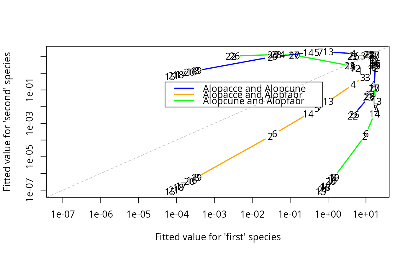
Trajectory plots can be defined in different ways for different models. Many models have no such notion or definition.

For quadratic and additive ordination models they plot the fitted values of two species against each other (more than two is theoretically possible, but not implemented in this software yet).

Value

The value returned depends specifically on the methods function invoked.

References

Yee, T. W. (2020). On constrained and unconstrained quadratic ordination. Manuscript in preparation.

Author

Thomas W. Yee

Examples

if (FALSE)  set.seed(123)
hspider[, 1:6] <- scale(hspider[, 1:6])  # Stdze environ. vars
p1cqo <- cqo(cbind(Alopacce, Alopcune, Alopfabr, Arctlute,
                   Arctperi, Auloalbi, Pardlugu, Pardmont,
                   Pardnigr, Pardpull, Trocterr, Zoraspin) ~
            WaterCon + BareSand + FallTwig +
            CoveMoss + CoveHerb + ReflLux,
            poissonff, data = hspider, Crow1positive = FALSE)
#> 
#> ========================= Fitting model 1 =========================
#> 
#> Obtaining initial values
#> 
#> Using initial values
#>          latvar
#> WaterCon -0.414
#> BareSand -0.984
#> FallTwig  1.484
#> CoveMoss -0.657
#> CoveHerb  0.439
#> ReflLux   0.197
#> 
#> Using BFGS algorithm
#> initial  value 2186.413676 
#> final  value 2157.494278 
#> converged
#> 
#> BFGS using optim(): 
#> Objective = 2157.494 
#> Parameters (= c(C)) =  
#> -0.02490175 0.1982131 -0.4557332 0.3012156 0.07304697 0.1761878
#> 
#> Number of function evaluations = 62 
#> 
#> 
#> ========================= Fitting model 2 =========================
#> 
#> Obtaining initial values
#> 
#> Using initial values
#>          latvar
#> WaterCon -0.186
#> BareSand  0.544
#> FallTwig -0.548
#> CoveMoss  0.569
#> CoveHerb -0.525
#> ReflLux   0.571
#> 
#> Using BFGS algorithm
#> initial  value 2375.995130 
#> iter  10 value 1585.128586
#> final  value 1585.128339 
#> converged
#> 
#> BFGS using optim(): 
#> Objective = 1585.128 
#> Parameters (= c(C)) =  
#> -0.1505028 0.2330187 -0.388664 0.1331737 -0.1293807 0.2967478
#> 
#> Number of function evaluations = 77 
#> 
#> 
#> ========================= Fitting model 3 =========================
#> 
#> Obtaining initial values
#> 
#> Using initial values
#>          latvar
#> WaterCon -0.145
#> BareSand  0.690
#> FallTwig -0.831
#> CoveMoss  0.484
#> CoveHerb -0.151
#> ReflLux   0.301
#> 
#> Using BFGS algorithm
#> initial  value 1653.157371 
#> iter  10 value 1585.121718
#> iter  10 value 1585.121718
#> iter  10 value 1585.121718
#> final  value 1585.121718 
#> converged
#> 
#> BFGS using optim(): 
#> Objective = 1585.122 
#> Parameters (= c(C)) =  
#> -0.1496598 0.2334462 -0.3886166 0.133672 -0.129245 0.2968041
#> 
#> Number of function evaluations = 81 
#> 
#> 
#> ========================= Fitting model 4 =========================
#> 
#> Obtaining initial values
#> 
#> Using initial values
#>          latvar
#> WaterCon -0.418
#> BareSand  0.762
#> FallTwig -0.520
#> CoveMoss  0.187
#> CoveHerb -0.148
#> ReflLux   0.515
#> 
#> Using BFGS algorithm
#> initial  value 1906.618242 
#> iter  10 value 1585.127710
#> iter  10 value 1585.127710
#> iter  10 value 1585.127710
#> final  value 1585.127710 
#> converged
#> 
#> BFGS using optim(): 
#> Objective = 1585.128 
#> Parameters (= c(C)) =  
#> -0.1506033 0.2330496 -0.3885228 0.1331366 -0.1293396 0.2967861
#> 
#> Number of function evaluations = 80 
#> 
#> 
#> ========================= Fitting model 5 =========================
#> 
#> Obtaining initial values
#> 
#> Using initial values
#>          latvar
#> WaterCon -0.450
#> BareSand  0.299
#> FallTwig -0.324
#> CoveMoss  0.686
#> CoveHerb -0.138
#> ReflLux   0.597
#> 
#> Using BFGS algorithm
#> initial  value 2154.083637 
#> iter  10 value 1585.127326
#> iter  10 value 1585.127326
#> iter  10 value 1585.127326
#> final  value 1585.127326 
#> converged
#> 
#> BFGS using optim(): 
#> Objective = 1585.127 
#> Parameters (= c(C)) =  
#> -0.1505215 0.2329896 -0.3885163 0.1333192 -0.1293691 0.2967641
#> 
#> Number of function evaluations = 108 
#> 
#> 
#> ========================= Fitting model 6 =========================
#> 
#> Obtaining initial values
#> 
#> Using initial values
#>           latvar
#> WaterCon -1.4182
#> BareSand  0.7037
#> FallTwig  0.2189
#> CoveMoss -0.5134
#> CoveHerb -0.8359
#> ReflLux  -0.0404
#> 
#> Using BFGS algorithm
#> initial  value 3032.172936 
#> iter  10 value 2472.115693
#> final  value 2472.062564 
#> converged
#> 
#> BFGS using optim(): 
#> Objective = 2472.063 
#> Parameters (= c(C)) =  
#> -0.8107649 0.07441269 0.4934273 0.1100099 -0.3474059 0.1344372
#> 
#> Number of function evaluations = 85 
#> 
#> 
#> ========================= Fitting model 7 =========================
#> 
#> Obtaining initial values
#> 
#> Using initial values
#>          latvar
#> WaterCon -0.484
#> BareSand  0.423
#> FallTwig -0.182
#> CoveMoss  0.235
#> CoveHerb -0.478
#> ReflLux   0.997
#> 
#> Using BFGS algorithm
#> initial  value 2605.491913 
#> iter  10 value 1600.660448
#> final  value 1585.126829 
#> converged
#> 
#> BFGS using optim(): 
#> Objective = 1585.127 
#> Parameters (= c(C)) =  
#> -0.1507643 0.2329362 -0.3884077 0.1332678 -0.1292034 0.2967033
#> 
#> Number of function evaluations = 95 
#> 
#> 
#> ========================= Fitting model 8 =========================
#> 
#> Obtaining initial values
#> 
#> Using initial values
#>          latvar
#> WaterCon -0.237
#> BareSand  0.389
#> FallTwig -0.559
#> CoveMoss  0.212
#> CoveHerb -0.500
#> ReflLux   0.975
#> 
#> Using BFGS algorithm
#> initial  value 1818.082109 
#> iter  10 value 1585.154494
#> final  value 1585.128635 
#> converged
#> 
#> BFGS using optim(): 
#> Objective = 1585.129 
#> Parameters (= c(C)) =  
#> -0.1505194 0.2330154 -0.3886991 0.1331877 -0.1293876 0.2966907
#> 
#> Number of function evaluations = 80 
#> 
#> 
#> ========================= Fitting model 9 =========================
#> 
#> Obtaining initial values
#> 
#> Using initial values
#>           latvar
#> WaterCon -1.6655
#> BareSand  0.0177
#> FallTwig  0.8715
#> CoveMoss -0.5700
#> CoveHerb -1.0760
#> ReflLux   0.4680
#> 
#> Using BFGS algorithm
#> initial  value 2850.861453 
#> iter  10 value 2472.163900
#> final  value 2472.066873 
#> converged
#> 
#> BFGS using optim(): 
#> Objective = 2472.067 
#> Parameters (= c(C)) =  
#> -0.8107955 0.0748189 0.4922993 0.1097398 -0.3475099 0.1334917
#> 
#> Number of function evaluations = 74 
#> 
#> 
#> ========================= Fitting model 10 =========================
#> 
#> Obtaining initial values
#> 
#> Using initial values
#>          latvar
#> WaterCon -0.265
#> BareSand  0.749
#> FallTwig -0.573
#> CoveMoss  0.200
#> CoveHerb -0.083
#> ReflLux   0.613
#> 
#> Using BFGS algorithm
#> initial  value 1808.194070 
#> iter  10 value 1585.137849
#> final  value 1585.128969 
#> converged
#> 
#> BFGS using optim(): 
#> Objective = 1585.129 
#> Parameters (= c(C)) =  
#> -0.1505216 0.2330105 -0.3887161 0.133204 -0.1294114 0.2966653
#> 
#> Number of function evaluations = 75 
#> 

nos <- ncol(depvar(p1cqo))
clr <- 1:nos  # OR (1:(nos+1))[-7]  to omit yellow

trplot(p1cqo, which.species = 1:3, log = "xy", lwd = 2,
       col = c("blue", "orange", "green"), label = TRUE) -> ii
legend(0.00005, 0.3, paste(ii$species[, 1], ii$species[, 2],
                           sep = " and "),
       lwd = 2, lty = 1, col = c("blue", "orange", "green"))
abline(a = 0, b = 1, lty = "dashed", col = "grey")  # \dontrun{}