Variability Summary: Statistics and Stylized Facts
Source:R/table.Variability.R
table.Variability.RdTable of Mean absolute difference, period standard deviation and annualised standard deviation
Arguments
- R
an xts, vector, matrix, data frame, timeSeries or zoo object of asset returns
- scale
number of periods in a year (daily scale = 252, monthly scale = 12, quarterly scale = 4)
- geometric
utilize geometric chaining (TRUE) or simple/arithmetic chaining (FALSE) to aggregate returns, default TRUE
- digits
number of digits to round results to
References
Carl Bacon, Practical portfolio performance measurement and attribution, second edition 2008 p.65
Examples
data(managers)
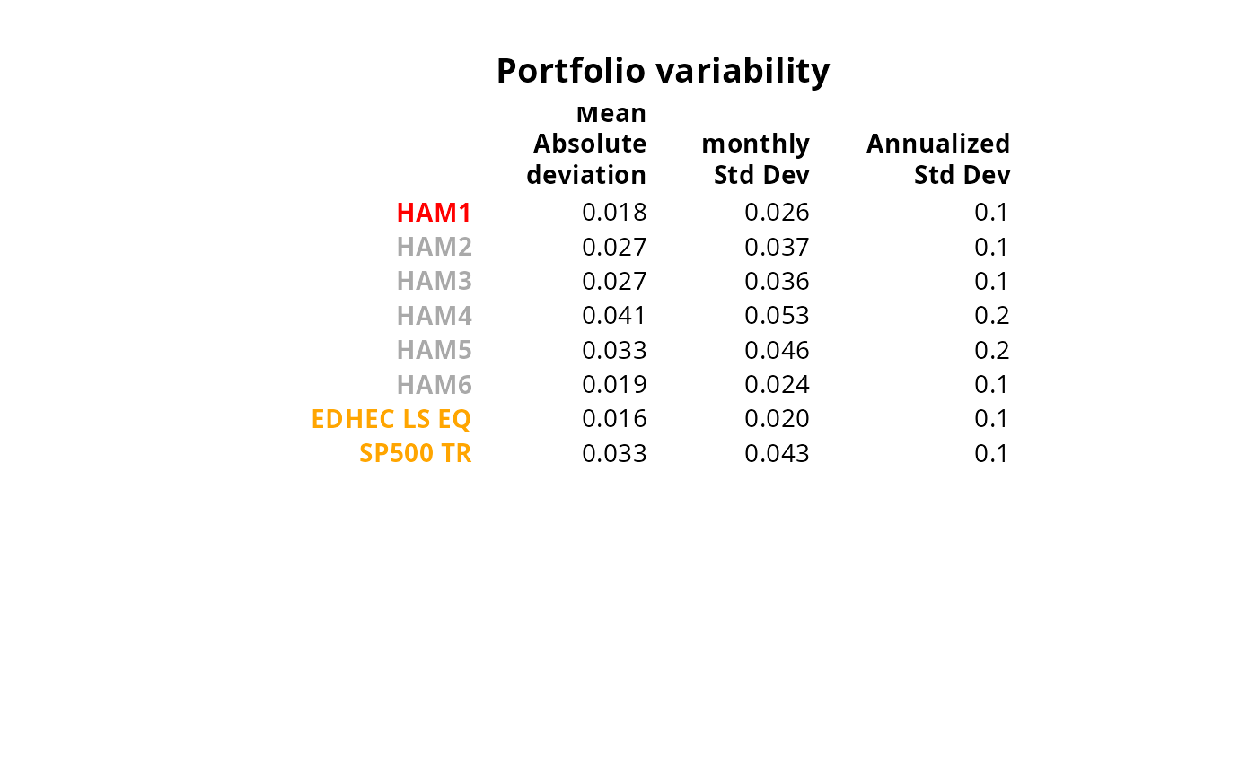
table.Variability(managers[, 1:8])
#> HAM1 HAM2 HAM3 HAM4 HAM5 HAM6 EDHEC LS EQ
#> Mean Absolute deviation 0.0182 0.0268 0.0268 0.0410 0.0329 0.0187 0.0159
#> monthly Std Dev 0.0256 0.0367 0.0365 0.0532 0.0457 0.0238 0.0205
#> Annualized Std Dev 0.0888 0.1272 0.1265 0.1843 0.1584 0.0825 0.0708
#> SP500 TR
#> Mean Absolute deviation 0.0333
#> monthly Std Dev 0.0433
#> Annualized Std Dev 0.1500
# \donttest{
# don't test on CRAN, since it requires Suggested packages
require("Hmisc")
result <- t(table.Variability(managers[, 1:8]))
textplot(format.df(result, na.blank = TRUE, numeric.dollar = FALSE, cdec = c(3, 3, 1)),
rmar = 0.8, cmar = 2, max.cex = .9, halign = "center", valign = "top",
row.valign = "center", wrap.rownames = 20, wrap.colnames = 10,
col.rownames = c("red", rep("darkgray", 5), rep("orange", 2)), mar = c(0, 0, 3, 0) + 0.1
)
title(main = "Portfolio variability")
 # }
# }