Single Factor Asset-Pricing Model Summary: Statistics and Stylized Facts
Source:R/table.CAPM.R
table.CAPM.RdTakes a set of returns and relates them to a benchmark return. Provides a set of measures related to an excess return single factor model, or CAPM.
table.SFM(Ra, Rb, scale = NA, Rf = 0, digits = 4)Arguments
- Ra
a vector of returns to test, e.g., the asset to be examined
- Rb
a matrix, data.frame, or timeSeries of benchmark(s) to test the asset against.
- scale
number of periods in a year (daily scale = 252, monthly scale = 12, quarterly scale = 4)
- Rf
risk free rate, in same period as your returns
- digits
number of digits to round results to
Details
This table will show statistics pertaining to an asset against a set of benchmarks, or statistics for a set of assets against a benchmark.
Examples
# CRAN does not allow examples to load suggested packages in one of its tests
data(managers)
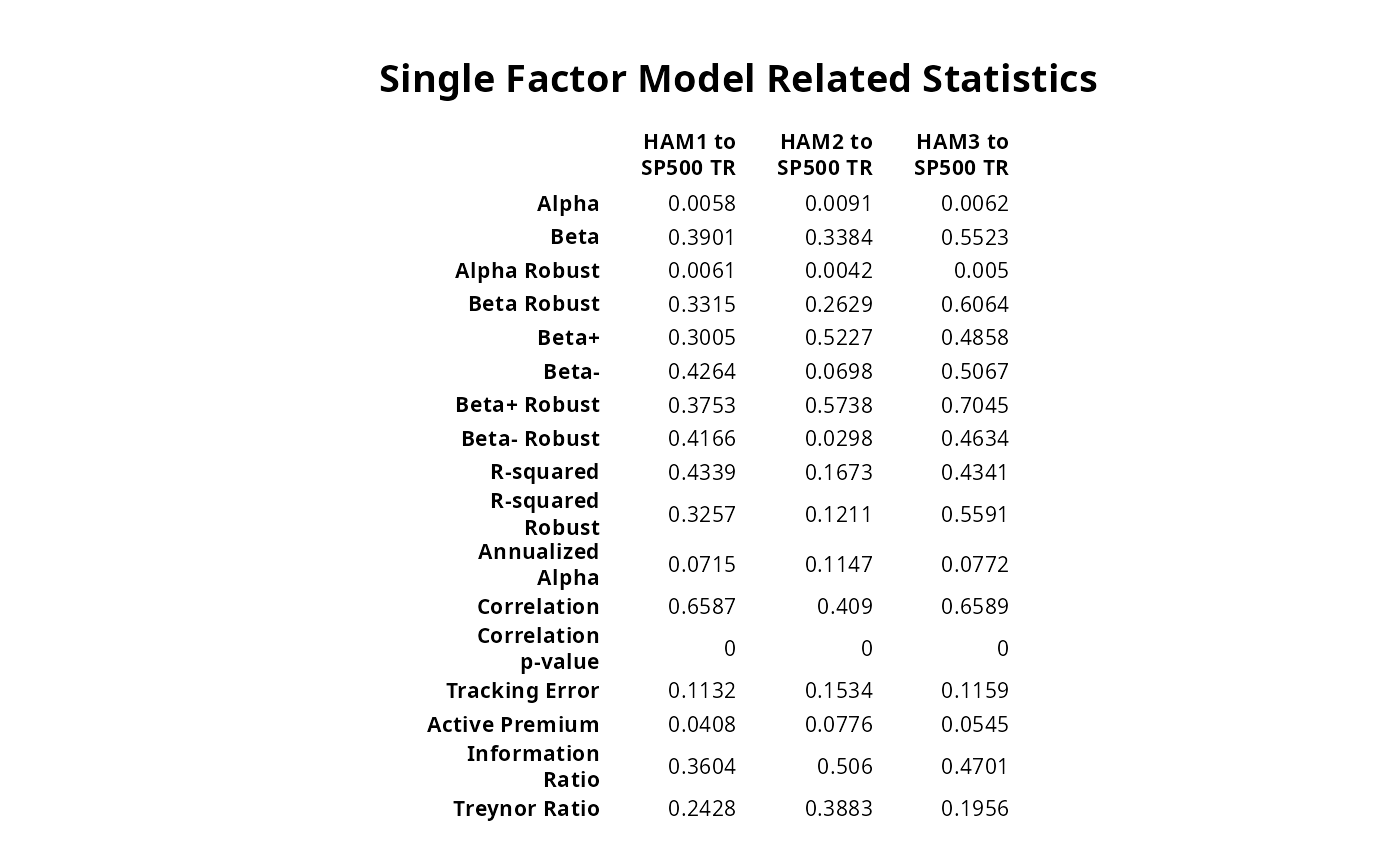
table.SFM(managers[,1:3], managers[,8], Rf = managers[,10])
#> HAM1 to SP500 TR HAM2 to SP500 TR HAM3 to SP500 TR
#> Alpha 0.0058 0.0091 0.0062
#> Beta 0.3901 0.3384 0.5523
#> Alpha Robust 0.0061 0.0042 0.0050
#> Beta Robust 0.3315 0.2629 0.6064
#> Beta+ 0.3005 0.5227 0.4858
#> Beta- 0.4264 0.0698 0.5067
#> Beta+ Robust 0.3753 0.5738 0.7045
#> Beta- Robust 0.4166 0.0298 0.4634
#> R-squared 0.4339 0.1673 0.4341
#> R-squared Robust 0.3257 0.1211 0.5591
#> Annualized Alpha 0.0715 0.1147 0.0772
#> Correlation 0.6587 0.4090 0.6589
#> Correlation p-value 0.0000 0.0000 0.0000
#> Tracking Error 0.1132 0.1534 0.1159
#> Active Premium 0.0408 0.0776 0.0545
#> Information Ratio 0.3604 0.5060 0.4701
#> Treynor Ratio 0.2428 0.3883 0.1956
result = table.SFM(managers[,1:3], managers[,8], Rf = managers[,10])
require(Hmisc)
textplot(result, rmar = 0.8, cmar = 1.5, max.cex=.9,
halign = "center", valign = "top", row.valign="center",
wrap.rownames=15, wrap.colnames=10, mar = c(0,0,3,0)+0.1)
title(main="Single Factor Model Related Statistics")