Calculate single factor model (CAPM) beta

The single factor model or CAPM Beta is the beta of an asset to the variance and covariance of an initial portfolio. Used to determine diversification potential.

SFM.beta(
  Ra,
  Rb,
  Rf = 0,
  ...,
  digits = 3,
  benchmarkCols = T,
  method = "LS",
  family = "mopt",
  warning = T
)

SFM.beta.bull(
  Ra,
  Rb,
  Rf = 0,
  ...,
  digits = 3,
  benchmarkCols = T,
  method = "LS",
  family = "mopt"
)

SFM.beta.bear(
  Ra,
  Rb,
  Rf = 0,
  ...,
  digits = 3,
  benchmarkCols = T,
  method = "LS",
  family = "mopt"
)

TimingRatio(Ra, Rb, Rf = 0, ...)

Arguments

Ra

an xts, vector, matrix, data frame, timeSeries or zoo object of asset returns

Rb

return vector of the benchmark asset

Rf

risk free rate, in same period as your returns

...

Other parameters like max.it or bb specific to lmrobdetMM regression.

digits

(Optional): Number of digits to round the results to. Defaults to 3.

benchmarkCols

(Optional): Boolean to show the benchmarks as columns. Defaults to TRUE.

method

(Optional): string representing linear regression model, "LS" for Least Squares and "Robust" for robust. Defaults to "LS

family

(Optional): If method == "Robust": This is a string specifying the name of the family of loss function to be used (current valid options are "bisquare", "opt" and "mopt"). Incomplete entries will be matched to the current valid options. Defaults to "mopt". Else: the parameter is ignored

warning

(Optional): Boolean to show warnings or not. Defaults to TRUE.

Details

This function uses a linear intercept model to achieve the same results as the symbolic model used by BetaCoVariance

$$\beta_{a,b}=\frac{CoV_{a,b}}{\sigma_{b}}=\frac{\sum((R_{a}-\bar{R_{a}})(R_{b}-\bar{R_{b}}))}{\sum(R_{b}-\bar{R_{b}})^{2}}$$

Ruppert(2004) reports that this equation will give the estimated slope of the linear regression of \(R_{a}\) on \(R_{b}\) and that this slope can be used to determine the risk premium or excess expected return (see Eq. 7.9 and 7.10, p. 230-231).

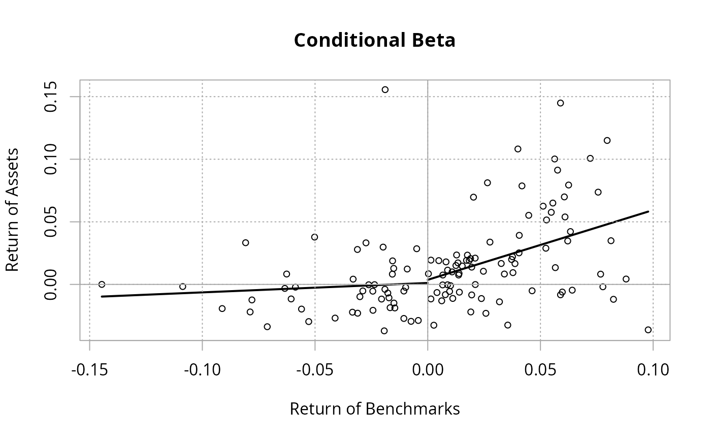
Two other functions apply the same notion of best fit to positive and negative market returns, separately. The SFM.beta.bull is a regression for only positive market returns, which can be used to understand the behavior of the asset or portfolio in positive or 'bull' markets. Alternatively, SFM.beta.bear provides the calculation on negative market returns.

The TimingRatio may help assess whether the manager is a good timer of asset allocation decisions. The ratio, which is calculated as $$TimingRatio =\frac{\beta^{+}}{\beta^{-}}$$ is best when greater than one in a rising market and less than one in a falling market.

While the classical CAPM has been almost completely discredited by the literature, it is an example of a simple single factor model, comparing an asset to any arbitrary benchmark.

References

Sharpe, W.F. Capital Asset Prices: A theory of market equilibrium under conditions of risk. Journal of finance, vol 19, 1964, 425-442.
Ruppert, David. Statistics and Finance, an Introduction. Springer. 2004.
Bacon, Carl. Practical portfolio performance measurement and attribution. Wiley. 2004.

See also

BetaCoVariance SFM.alpha CAPM.utils

Author

Dhairya Jain, Peter Carl

Examples

data(managers)

SFM.beta(managers[, "HAM1"], managers[, "SP500 TR"], Rf = managers[, "US 3m TR"])
#> [1] 0.3900712
SFM.beta(managers[,1:3], managers[,8:10], Rf=.035/12) 
#>      Beta : SP500 TR Beta : US 10Y TR Beta : US 3m TR
#> HAM1           0.391           -0.359           0.692
#> HAM2           0.343           -0.043           4.159
#> HAM3           0.557           -0.099           4.687
SFM.beta(managers[,1], managers[,8:10], Rf=.035/12, benchmarkCols=FALSE) 
#>                    HAM1
#> Beta : SP500 TR   0.391
#> Beta : US 10Y TR -0.359
#> Beta : US 3m TR   0.692

SFM.beta.bull(managers[, "HAM2"], 
               managers[, "SP500 TR"], 
               Rf = managers[, "US 3m TR"])
#> [1] 0.5226596
               
SFM.beta.bear(managers[, "HAM2"], 
               managers[, "SP500 TR"], 
               Rf = managers[, "US 3m TR"])
#> [1] 0.0698255
      
TimingRatio(managers[, "HAM2"], 
             managers[, "SP500 TR"], 
             Rf = managers[, "US 3m TR"])
#> [1] 7.485224
      
if(requireNamespace("RobStatTM", quietly = TRUE)) { # CRAN requires conditional execution
  betas <- SFM.beta(managers[,1:6], 
                     managers[,8:10], 
                     Rf=.035/12, method="Robust", 
                     family="opt", bb=0.25, max.it=200, digits=4)
   betas["HAM1", ]
   betas[, "Beta : SP500 TR"]
       
  SFM.beta.bull(managers[, "HAM2"], 
                 managers[, "SP500 TR"], 
                 Rf = managers[, "US 3m TR"],
                 method="Robust")
      
  SFM.beta.bear(managers[, "HAM2"], 
                 managers[, "SP500 TR"], 
                 Rf = managers[, "US 3m TR"],
                 method="Robust")
                 
   TimingRatio(managers[, "HAM2"], 
                managers[, "SP500 TR"], 
               Rf = managers[, "US 3m TR"],
               method="Robust", family="mopt")
      
} # CRAN can have issues with RobStatTM
#> [1] 19.26492
      
chart.Regression(managers[, "HAM2"], 
                  managers[, "SP500 TR"], 
                  Rf = managers[, "US 3m TR"], 
                  fit="conditional", 
                  main="Conditional Beta")