Nearest Positive Definite Matrix

Compute the nearest positive definite matrix to an approximate one, typically a correlation or variance-covariance matrix.

Usage

nearPD(x, corr = FALSE, keepDiag = FALSE, base.matrix = FALSE,
       do2eigen = TRUE, doSym = FALSE,
       doDykstra = TRUE, only.values = FALSE,
       ensureSymmetry = !isSymmetric(x),
       eig.tol = 1e-06, conv.tol = 1e-07, posd.tol = 1e-08,
       maxit = 100, conv.norm.type = "I", trace = FALSE)

Arguments

x: numeric \(n \times n\) approximately positive definite matrix, typically an approximation to a correlation or covariance matrix. If x is not symmetric (and ensureSymmetry is not false), symmpart(x) is used.
corr: logical indicating if the matrix should be a correlation matrix.
keepDiag: logical, generalizing corr: if TRUE, the resulting matrix should have the same diagonal (diag(x)) as the input matrix.
base.matrix: logical indicating if the resulting mat component should be a base matrix or (by default) a Matrix of class dpoMatrix.
do2eigen: logical indicating if a posdefify() eigen step should be applied to the result of the Higham algorithm.
doSym: logical indicating if X <- (X + t(X))/2 should be done, after X <- tcrossprod(Qd, Q); some doubt if this is necessary.
doDykstra: logical indicating if Dykstra's correction should be used; true by default. If false, the algorithm is basically the direct fixpoint iteration \(Y_k = P_U(P_S(Y_{k-1}))\).
only.values: logical; if TRUE, the result is just the vector of eigenvalues of the approximating matrix.
ensureSymmetry: logical; by default, symmpart(x) is used whenever isSymmetric(x) is not true. The user can explicitly set this to TRUE or FALSE, saving the symmetry test. Beware however that setting it FALSE for an asymmetric input x, is typically nonsense!
eig.tol: defines relative positiveness of eigenvalues compared to largest one, \(\lambda_1\). Eigenvalues \(\lambda_k\) are treated as if zero when \(\lambda_k / \lambda_1 \le eig.tol\).
conv.tol: convergence tolerance for Higham algorithm.
posd.tol: tolerance for enforcing positive definiteness (in the final posdefify step when do2eigen is TRUE).
maxit: maximum number of iterations allowed.
conv.norm.type: convergence norm type (norm(*, type)) used for Higham algorithm. The default is "I" (infinity), for reasons of speed (and back compatibility); using "F" is more in line with Higham's proposal.
trace: logical or integer specifying if convergence monitoring should be traced.

Details

This implements the algorithm of Higham (2002), and then (if do2eigen is true) forces positive definiteness using code from posdefify. The algorithm of Knol and ten Berge (1989) (not implemented here) is more general in that it allows constraints to (1) fix some rows (and columns) of the matrix and (2) force the smallest eigenvalue to have a certain value.

Note that setting corr = TRUE just sets diag(.) <- 1 within the algorithm.

Higham (2002) uses Dykstra's correction, but the version by Jens Oehlschlägel did not use it (accidentally), and still gave reasonable results; this simplification, now only used if doDykstra = FALSE, was active in nearPD() up to Matrix version 0.999375-40.

Value

If only.values = TRUE, a numeric vector of eigenvalues of the approximating matrix; Otherwise, as by default, an S3 object of class "nearPD", basically a list with components

mat: a matrix of class dpoMatrix, the computed positive-definite matrix.
eigenvalues: numeric vector of eigenvalues of mat.
corr: logical, just the argument corr.
normF: the Frobenius norm (norm(x-X, "F")) of the difference between the original and the resulting matrix.
iterations: number of iterations needed.
converged: logical indicating if iterations converged.

References

Cheng, Sheung Hun and Higham, Nick (1998) A Modified Cholesky Algorithm Based on a Symmetric Indefinite Factorization; SIAM J. Matrix Anal.\ Appl., 19, 1097–1110.

Knol DL, ten Berge JMF (1989) Least-squares approximation of an improper correlation matrix by a proper one. Psychometrika 54, 53–61.

Higham, Nick (2002) Computing the nearest correlation matrix - a problem from finance; IMA Journal of Numerical Analysis 22, 329–343.

Author

Jens Oehlschlägel donated a first version. Subsequent changes by the Matrix package authors.

Examples

 ## Higham(2002), p.334f - simple example
 A <- matrix(1, 3,3); A[1,3] <- A[3,1] <- 0
 n.A <- nearPD(A, corr=TRUE, do2eigen=FALSE)
 n.A[c("mat", "normF")]
#> $mat
#> 3 x 3 Matrix of class "dpoMatrix"
#>           [,1]      [,2]      [,3]
#> [1,] 1.0000000 0.7606899 0.1572981
#> [2,] 0.7606899 1.0000000 0.7606899
#> [3,] 0.1572981 0.7606899 1.0000000
#> 
#> $normF
#> [1] 0.5277903
#> 
 n.A.m <- nearPD(A, corr=TRUE, do2eigen=FALSE, base.matrix=TRUE)$mat
 stopifnot(exprs = {                           #=--------------
   all.equal(n.A$mat[1,2], 0.760689917)
   all.equal(n.A$normF, 0.52779033, tolerance=1e-9)
   all.equal(n.A.m, unname(as.matrix(n.A$mat)), tolerance = 1e-15)# seen rel.d.= 1.46e-16
 })
 set.seed(27)
 m <- matrix(round(rnorm(25),2), 5, 5)
 m <- m + t(m)
 diag(m) <- pmax(0, diag(m)) + 1
 (m <- round(cov2cor(m), 2))
#>       [,1]  [,2]  [,3]  [,4]  [,5]
#> [1,]  1.00  0.65 -0.46 -1.15 -0.76
#> [2,]  0.65  1.00  0.58  0.50 -0.90
#> [3,] -0.46  0.58  1.00 -0.45 -0.32
#> [4,] -1.15  0.50 -0.45  1.00  0.25
#> [5,] -0.76 -0.90 -0.32  0.25  1.00

 str(near.m <- nearPD(m, trace = TRUE))
#> iter   1 : #{p}=4, ||Y-X|| / ||Y||=    0.268591
#> iter   2 : #{p}=4, ||Y-X|| / ||Y||=           0
#> List of 7
#>  $ mat        :Formal class 'dpoMatrix' [package "Matrix"] with 5 slots
#>   .. ..@ Dim     : int [1:2] 5 5
#>   .. ..@ Dimnames:List of 2
#>   .. .. ..$ : NULL
#>   .. .. ..$ : NULL
#>   .. ..@ x       : num [1:25] 1.313 0.406 -0.242 -0.852 -0.753 ...
#>   .. ..@ uplo    : chr "U"
#>   .. ..@ factors : list()
#>  $ eigenvalues: num [1:5] 2.80 1.83 1.23 7.70e-02 2.80e-08
#>  $ corr       : logi FALSE
#>  $ normF      : num 0.938
#>  $ iterations : int 2
#>  $ rel.tol    : num 0
#>  $ converged  : logi TRUE
#>  - attr(*, "class")= chr "nearPD"
 round(near.m$mat, 2)
#> 5 x 5 Matrix of class "dsyMatrix"
#>       [,1]  [,2]  [,3]  [,4]  [,5]
#> [1,]  1.31  0.41 -0.24 -0.85 -0.75
#> [2,]  0.41  1.19  0.41  0.27 -0.91
#> [3,] -0.24  0.41  1.15 -0.24 -0.32
#> [4,] -0.85  0.27 -0.24  1.28  0.26
#> [5,] -0.75 -0.91 -0.32  0.26  1.00
 norm(m - near.m$mat) # 1.102 / 1.08
#> [1] 1.079735

 if(requireNamespace("sfsmisc")) {
    m2 <- sfsmisc::posdefify(m) # a simpler approach
    norm(m - m2)  # 1.185, i.e., slightly "less near"
 }
#> Loading required namespace: sfsmisc
#> [1] 1.184855

 round(nearPD(m, only.values=TRUE), 9)
#> [1] 2.800681404 1.831722441 1.229003616 0.076994641 0.000000028

## A longer example, extended from Jens' original,
## showing the effects of some of the options:

pr <- Matrix(c(1,     0.477, 0.644, 0.478, 0.651, 0.826,
               0.477, 1,     0.516, 0.233, 0.682, 0.75,
               0.644, 0.516, 1,     0.599, 0.581, 0.742,
               0.478, 0.233, 0.599, 1,     0.741, 0.8,
               0.651, 0.682, 0.581, 0.741, 1,     0.798,
               0.826, 0.75,  0.742, 0.8,   0.798, 1),
             nrow = 6, ncol = 6)

nc.  <- nearPD(pr, conv.tol = 1e-7) # default
nc.$iterations  # 2
#> [1] 2
nc.1 <- nearPD(pr, conv.tol = 1e-7, corr = TRUE)
nc.1$iterations # 11 / 12 (!)
#> [1] 12
ncr   <- nearPD(pr, conv.tol = 1e-15)
str(ncr)# still 2 iterations
#> List of 7
#>  $ mat        :Formal class 'dpoMatrix' [package "Matrix"] with 5 slots
#>   .. ..@ Dim     : int [1:2] 6 6
#>   .. ..@ Dimnames:List of 2
#>   .. .. ..$ : NULL
#>   .. .. ..$ : NULL
#>   .. ..@ x       : num [1:36] 1.006 0.485 0.643 0.487 0.646 ...
#>   .. ..@ uplo    : chr "U"
#>   .. ..@ factors : list()
#>  $ eigenvalues: num [1:6] 4.213 0.771 0.515 0.385 0.178 ...
#>  $ corr       : logi FALSE
#>  $ normF      : num 0.0626
#>  $ iterations : int 2
#>  $ rel.tol    : num 0
#>  $ converged  : logi TRUE
#>  - attr(*, "class")= chr "nearPD"
ncr.1 <- nearPD(pr, conv.tol = 1e-15, corr = TRUE)
ncr.1 $ iterations # 27 / 30 !
#> [1] 31

ncF <- nearPD(pr, conv.tol = 1e-15, conv.norm = "F")
stopifnot(all.equal(ncr, ncF))# norm type does not matter at all in this example

## But indeed, the 'corr = TRUE' constraint did ensure a better solution;
## cov2cor() does not just fix it up equivalently :
norm(pr - cov2cor(ncr$mat)) # = 0.09994
#> [1] 0.09994443
norm(pr -       ncr.1$mat)  # = 0.08746 / 0.08805
#> [1] 0.08804689

### 3) a real data example from a 'systemfit' model (3 eq.):
(load(system.file("external", "symW.rda", package="Matrix"))) # "symW"
#> [1] "symW"
dim(symW) #  24 x 24
#> [1] 24 24
class(symW)# "dsCMatrix": sparse symmetric
#> [1] "dsCMatrix"
#> attr(,"package")
#> [1] "Matrix"
if(dev.interactive())  image(symW)
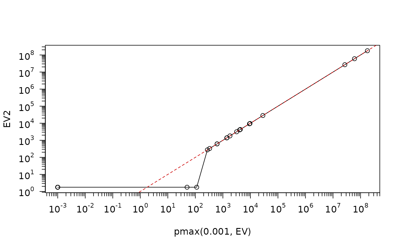
EV <- eigen(symW, only=TRUE)$values
summary(EV) ## looking more closely {EV sorted decreasingly}:
#>      Min.   1st Qu.    Median      Mean   3rd Qu.      Max. 
#>         0        37       999  11031812      5536 177467251 
tail(EV)# all 6 are negative
#> [1] -1.615418e-05 -4.803894e-05 -9.448841e-05 -8.402689e-04 -1.658025e-03
#> [6] -5.476273e-03
EV2 <- eigen(sWpos <- nearPD(symW)$mat, only=TRUE)$values
stopifnot(EV2 > 0)
if(requireNamespace("sfsmisc")) {
    plot(pmax(1e-3,EV), EV2, type="o", log="xy", xaxt="n", yaxt="n")
    for(side in 1:2) sfsmisc::eaxis(side)
} else
    plot(pmax(1e-3,EV), EV2, type="o", log="xy")
abline(0, 1, col="red3", lty=2)