Methods for image() in Package 'Matrix'
image-methods.RdMethods for function image in package
Matrix. An image of a matrix simply color codes all matrix
entries and draws the \(n\times m\) matrix using an
\(n\times m\) grid of (colored) rectangles.
The Matrix package image methods are based on
levelplot() from package lattice; hence
these methods return an “object” of class "trellis",
producing a graphic when (auto-) print()ed.
Usage
<!-- % want \usage{} since we have many "surprising arguments" -->
# S4 method for class 'dgTMatrix'
image(x,
      xlim = c(1, di[2]),
      ylim = c(di[1], 1), aspect = "iso",
      sub = sprintf("Dimensions: %d x %d", di[1], di[2]),
      xlab = "Column", ylab = "Row", cuts = 15,
      useRaster = FALSE,
      useAbs = NULL, colorkey = !useAbs,
      col.regions = NULL,
      lwd = NULL, border.col = NULL, ...)
Arguments
- x
a Matrix object, i.e., fulfilling
is(x, "Matrix").- xlim, ylim
x- and y-axis limits; may be used to “zoom into” matrix. Note that \(x,y\) “feel reversed”:
ylimis for the rows (= 1st index) andxlimfor the columns (= 2nd index). For convenience, when the limits are integer valued, they are both extended by0.5; also,ylimis always used decreasingly.- aspect
aspect ratio specified as number (y/x) or string; see
levelplot.- sub, xlab, ylab
axis annotation with sensible defaults; see
plot.default.- cuts
number of levels the range of matrix values would be divided into.
- useRaster
logical indicating if raster graphics should be used (instead of the tradition rectangle vector drawing). If true,
panel.levelplot.raster(from lattice package) is used, and the colorkey is also done via rasters, see alsolevelplotand possiblygrid.raster.Note that using raster graphics may often be faster, but can be slower, depending on the matrix dimensions and the graphics device (dimensions).
- useAbs
logical indicating if
abs(x)should be shown; ifTRUE, the former (implicit) default, the defaultcol.regionswill begreycolors (and nocolorkeydrawn). The default isFALSEunless the matrix has no negative entries.- colorkey
logical indicating if a color key aka ‘legend’ should be produced. Default is to draw one, unless
useAbsis true. You can also specify alist, seelevelplot, such aslist(raster=TRUE)in the case of rastering.- col.regions
vector of gradually varying colors; see
levelplot.- lwd
(only used when
useRasteris false:) non-negative number orNULL(default), specifying the line-width of the rectangles of each non-zero matrix entry (drawn bygrid.rect). The default depends on the matrix dimension and the device size.- border.col
color for the border of each rectangle.
NAmeans no border is drawn. WhenNULLas by default,border.col <- if(lwd < .01) NA else NULLis used. Consider using an opaque color instead ofNULLwhich corresponds togrid::get.gpar("col").- ...
further arguments passed to methods and
levelplot, notablyatfor specifying (possibly non equidistant) cut values for dividing the matrix values (supersedingcutsabove).
Methods
All methods currently end up calling the method for the
dgTMatrix class.
Use showMethods(image) to list them all.
Value
as all lattice graphics functions, image(<Matrix>)
returns a "trellis" object, effectively the result of
levelplot().
See also
levelplot, and
print.trellis from package lattice.
Examples
showMethods(image)
#> Function: image (package graphics)
#> x="ANY"
#> x="CHMfactor"
#> x="Matrix"
#> x="dgTMatrix"
#> x="matrix.csr"
#>
## And if you want to see the method definitions:
showMethods(image, includeDefs = TRUE, inherited = FALSE)
#> Function: image (package graphics)
#> x="ANY"
#> function (x, ...)
#> UseMethod("image")
#>
#>
#> x="CHMfactor"
#> function (x, ...)
#> image(.M2gen(.M2T(expand1(x, "L"))), ...)
#>
#>
#> x="Matrix"
#> function (x, ...)
#> {
#> if (.M.kind(x) == "z")
#> stop(gettextf("%s(<%s>) is not yet implemented", "image",
#> "zMatrix"), domain = NA)
#> image(.M2kind(.M2gen(.M2T(x)), "d"), ...)
#> }
#>
#>
#> x="dgTMatrix"
#> function (x, ...)
#> {
#> .local <- function (x, xlim = c(1, di[2L]), ylim = c(di[1L],
#> 1), aspect = "iso", sub = sprintf("Dimensions: %d x %d",
#> di[1L], di[2L]), xlab = "Column", ylab = "Row", cuts = 15,
#> useRaster = FALSE, useAbs = NULL, colorkey = !useAbs,
#> col.regions = NULL, lwd = NULL, border.col = NULL, ...)
#> {
#> di <- x@Dim
#> xx <- x@x
#> empty.x <- length(xx) == 0L && length(x) > 0L
#> if (empty.x) {
#> xx <- 0
#> x@i <- x@j <- 0L
#> }
#> if (missing(useAbs))
#> useAbs <- if (empty.x)
#> FALSE
#> else min(xx, na.rm = TRUE) >= 0
#> else if (useAbs)
#> xx <- abs(xx)
#> if (is.null(col.regions)) {
#> l.col <- empty.x || diff(rx <- range(xx, finite = TRUE)) ==
#> 0
#> col.regions <- if (useAbs) {
#> grey(if (l.col)
#> 0.9
#> else seq(from = 0.7, to = 0, length.out = 100L))
#> }
#> else if (l.col)
#> "gray90"
#> else {
#> nn <- 100
#> n0 <- min(nn, max(0, round((0 - rx[1L])/(rx[2L] -
#> rx[1L]) * nn)))
#> col.regions <- c(colorRampPalette(c("blue3",
#> "gray80"))(n0), colorRampPalette(c("gray75",
#> "red3"))(nn - n0))
#> }
#> }
#> if (!is.null(lwd) && !(is.numeric(lwd) && all(lwd >=
#> 0)))
#> stop("'lwd' must be NULL or non-negative numeric")
#> stopifnot(length(xlim) == 2L, length(ylim) == 2L)
#> ylim <- sort(ylim, decreasing = TRUE)
#> if (all(xlim == round(xlim)))
#> xlim <- xlim + c(-0.5, +0.5)
#> if (all(ylim == round(ylim)))
#> ylim <- ylim + c(+0.5, -0.5)
#> panel <- if (useRaster)
#> panel.levelplot.raster
#> else {
#> function(x, y, z, subscripts, at, ..., col.regions) {
#> x <- as.numeric(x[subscripts])
#> y <- as.numeric(y[subscripts])
#> numcol <- length(at) - 1L
#> num.r <- length(col.regions)
#> col.regions <- if (num.r <= numcol)
#> rep_len(col.regions, numcol)
#> else col.regions[1 + ((1:numcol - 1) * (num.r -
#> 1))%/%(numcol - 1)]
#> zcol <- rep.int(NA_integer_, length(z))
#> for (i in seq_along(col.regions)) zcol[!is.na(x) &
#> !is.na(y) & !is.na(z) & at[i] <= z & z < at[i +
#> 1L]] <- i
#> zcol <- zcol[subscripts]
#> if (any(subscripts)) {
#> if (is.null(lwd)) {
#> wh <- current.viewport()[c("width", "height")]
#> wh <- (par("cra")/par("cin")) * c(convertWidth(wh$width,
#> "inches", valueOnly = TRUE), convertHeight(wh$height,
#> "inches", valueOnly = TRUE))
#> pSize <- wh/di
#> pA <- prod(pSize)
#> p1 <- min(pSize)
#> lwd <- if (p1 < 2 || pA < 6)
#> 0.01
#> else if (p1 >= 4)
#> 1
#> else if (p1 > 3)
#> 0.5
#> else 0.2
#> Matrix.message("rectangle size ", paste(round(pSize,
#> 1L), collapse = " x "), " [pixels]; --> lwd :",
#> formatC(lwd))
#> }
#> else stopifnot(is.numeric(lwd), all(lwd >=
#> 0))
#> if (is.null(border.col) && lwd < 0.01)
#> border.col <- NA
#> grid.rect(x = x, y = y, width = 1, height = 1,
#> default.units = "native", gp = gpar(fill = col.regions[zcol],
#> lwd = lwd, col = border.col))
#> }
#> }
#> }
#> levelplot(xx ~ (x@j + 1L) * (x@i + 1L), sub = sub, xlab = xlab,
#> ylab = ylab, xlim = xlim, ylim = ylim, aspect = aspect,
#> colorkey = colorkey, col.regions = col.regions, cuts = cuts,
#> par.settings = list(background = list(col = "transparent")),
#> panel = panel, ...)
#> }
#> .local(x, ...)
#> }
#>
#>
#> x="matrix.csr"
#> function (x, ...)
#> {
#> .local <- function (x, col = c("white", "gray"), xlab = "column",
#> ylab = "row", ...)
#> {
#> n <- x@dimension[1]
#> p <- x@dimension[2]
#> z <- matrix(0, n, p)
#> column <- x@ja
#> row <- rep(n:1, diff(x@ia))
#> z[cbind(row, column)] <- 1
#> image.default(x = 1:p, y = -(n:1), t(z), axes = FALSE,
#> col = col, xlab = xlab, ylab = ylab, ...)
#> axis(1, pretty(1:p), ...)
#> axis(2, pretty(-(n:1)), labels = rev(pretty(1:n)), ...)
#> box()
#> }
#> .local(x, ...)
#> }
#>
#>
#>
data(CAex, package = "Matrix")
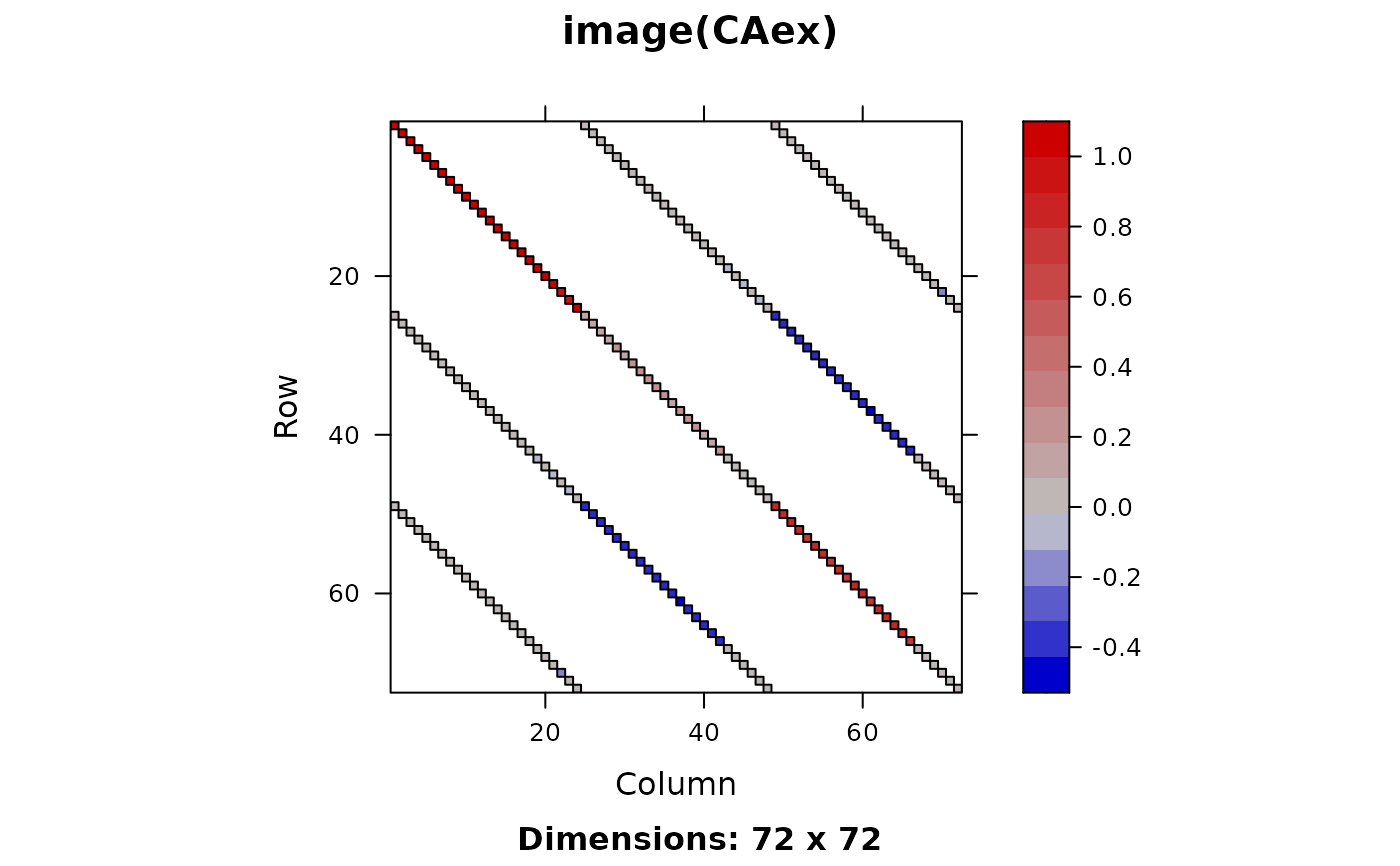
image(CAex, main = "image(CAex)") -> imgC; imgC
 stopifnot(!is.null(leg <- imgC$legend), is.list(leg$right)) # failed for 2 days ..
image(CAex, useAbs=TRUE, main = "image(CAex, useAbs=TRUE)")
stopifnot(!is.null(leg <- imgC$legend), is.list(leg$right)) # failed for 2 days ..
image(CAex, useAbs=TRUE, main = "image(CAex, useAbs=TRUE)")
 cCA <- Cholesky(crossprod(CAex), Imult = .01)
## See ?print.trellis --- place two image() plots side by side:
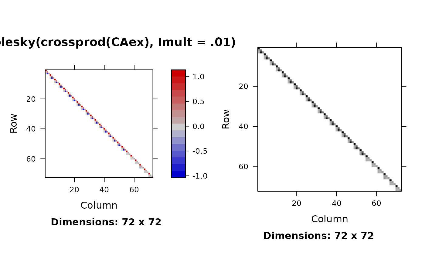
print(image(cCA, main="Cholesky(crossprod(CAex), Imult = .01)"),
split=c(x=1,y=1,nx=2, ny=1), more=TRUE)
print(image(cCA, useAbs=TRUE),
split=c(x=2,y=1,nx=2,ny=1))
cCA <- Cholesky(crossprod(CAex), Imult = .01)
## See ?print.trellis --- place two image() plots side by side:
print(image(cCA, main="Cholesky(crossprod(CAex), Imult = .01)"),
split=c(x=1,y=1,nx=2, ny=1), more=TRUE)
print(image(cCA, useAbs=TRUE),
split=c(x=2,y=1,nx=2,ny=1))
 data(USCounties, package = "Matrix")
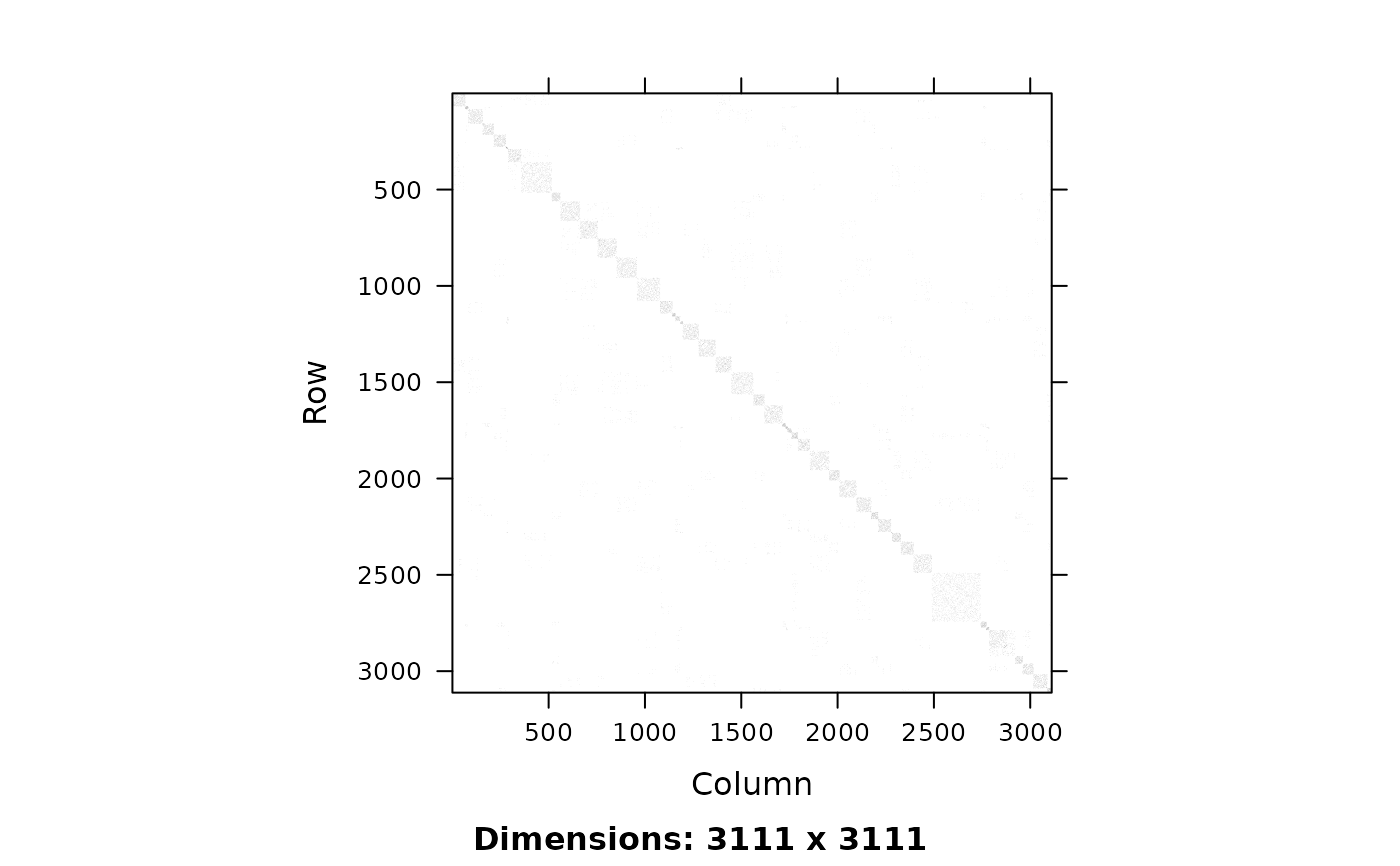
image(USCounties)# huge
data(USCounties, package = "Matrix")
image(USCounties)# huge
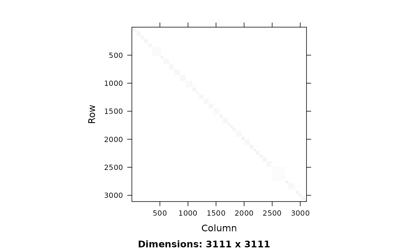
 image(sign(USCounties))## just the pattern
 # how the result looks, may depend heavily on
# the device, screen resolution, antialiasing etc
# e.g. x11(type="Xlib") may show very differently than cairo-based
## Drawing borders around each rectangle;
# again, viewing depends very much on the device:
image(USCounties[1:400,1:200], lwd=.1)
# how the result looks, may depend heavily on
# the device, screen resolution, antialiasing etc
# e.g. x11(type="Xlib") may show very differently than cairo-based
## Drawing borders around each rectangle;
# again, viewing depends very much on the device:
image(USCounties[1:400,1:200], lwd=.1)
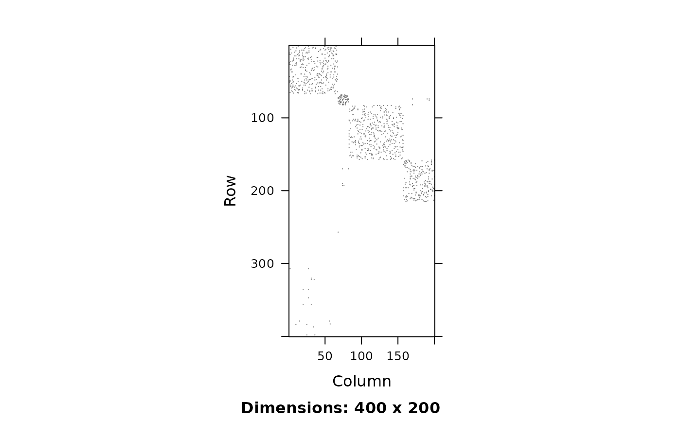 ## Using (xlim,ylim) has advantage : matrix dimension and (col/row) indices:
image(USCounties, c(1,200), c(1,400), lwd=.1)
## Using (xlim,ylim) has advantage : matrix dimension and (col/row) indices:
image(USCounties, c(1,200), c(1,400), lwd=.1)
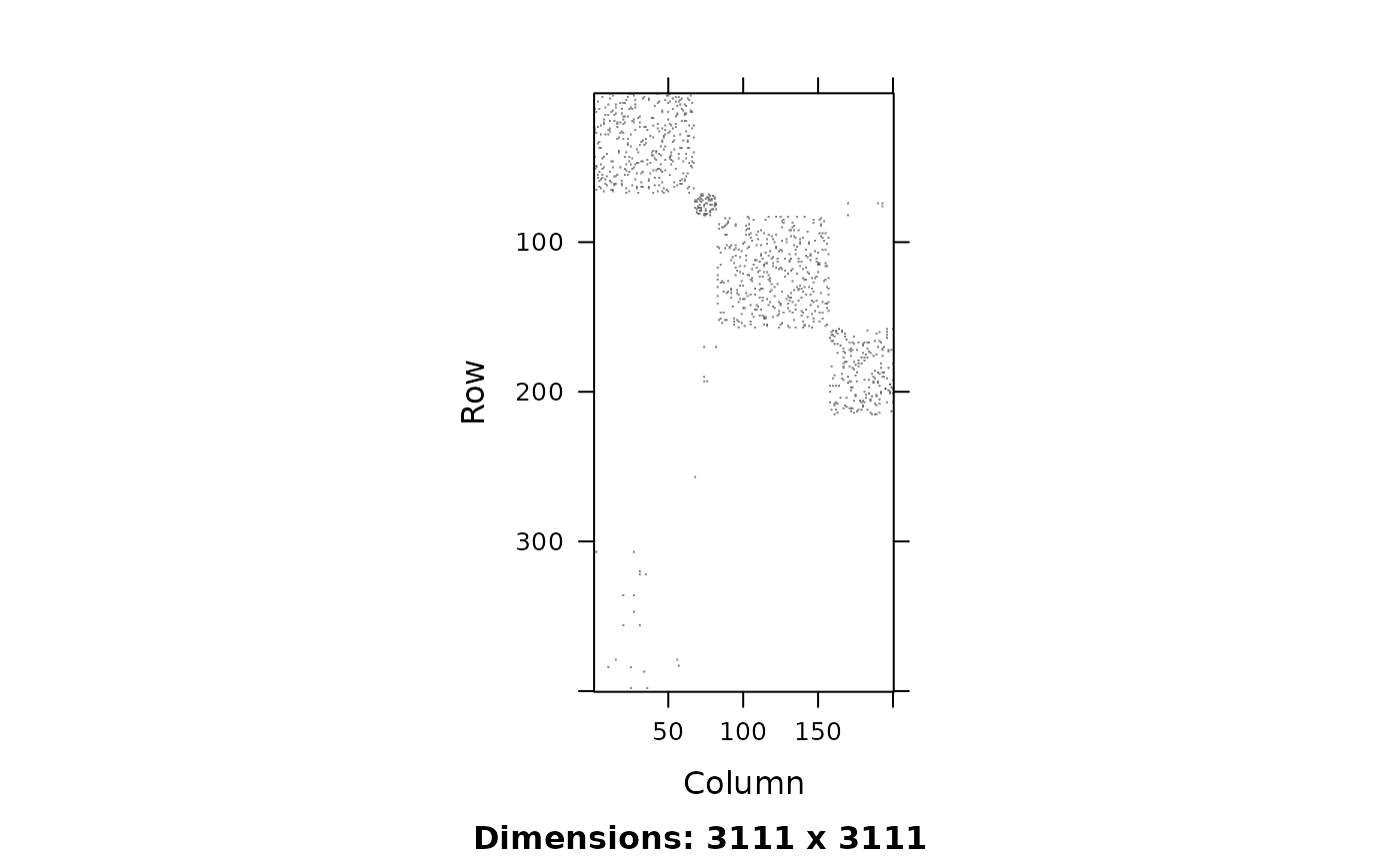 image(USCounties, c(1,300), c(1,200), lwd=.5 )
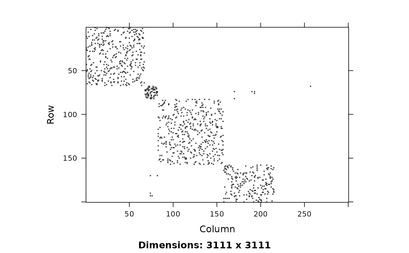 image(USCounties, c(1,300), c(1,200), lwd=.01)
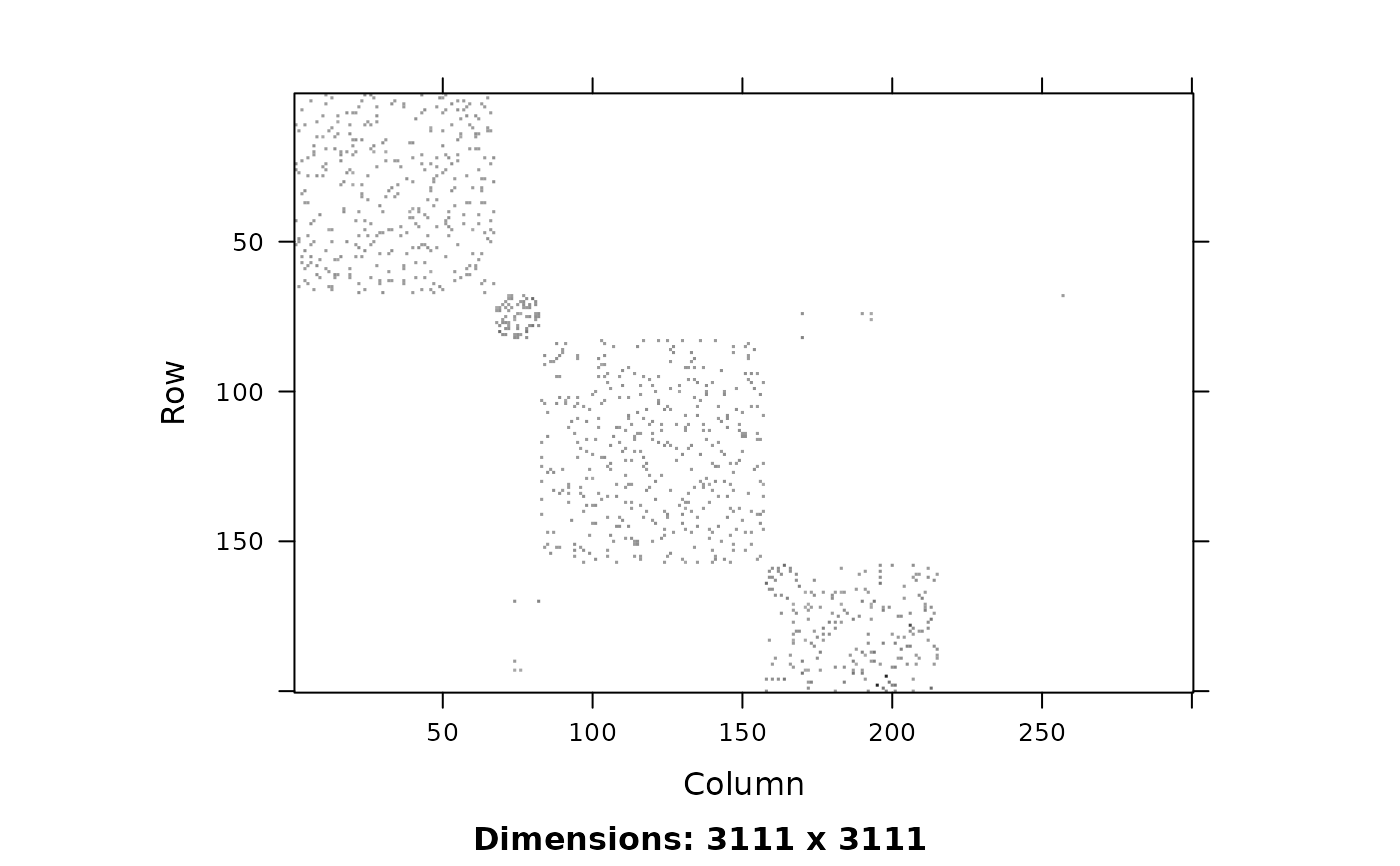 ## These 3 are all equivalent :
(I1 <- image(USCounties, c(1,100), c(1,100), useAbs=FALSE))
## These 3 are all equivalent :
(I1 <- image(USCounties, c(1,100), c(1,100), useAbs=FALSE))
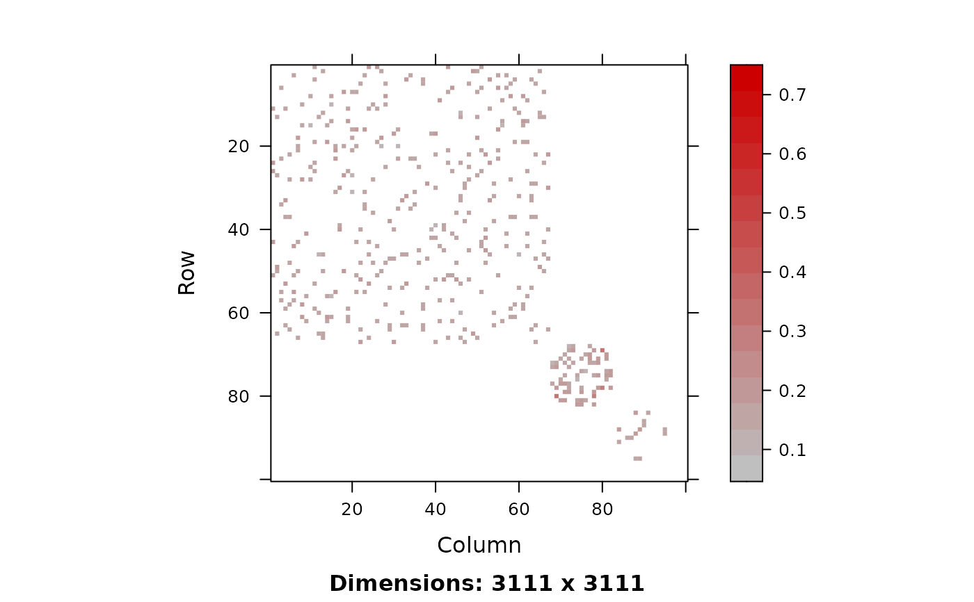 I2 <- image(USCounties, c(1,100), c(1,100), useAbs=FALSE, border.col=NA)
I3 <- image(USCounties, c(1,100), c(1,100), useAbs=FALSE, lwd=2, border.col=NA)
stopifnot(all.equal(I1, I2, check.environment=FALSE),
all.equal(I2, I3, check.environment=FALSE))
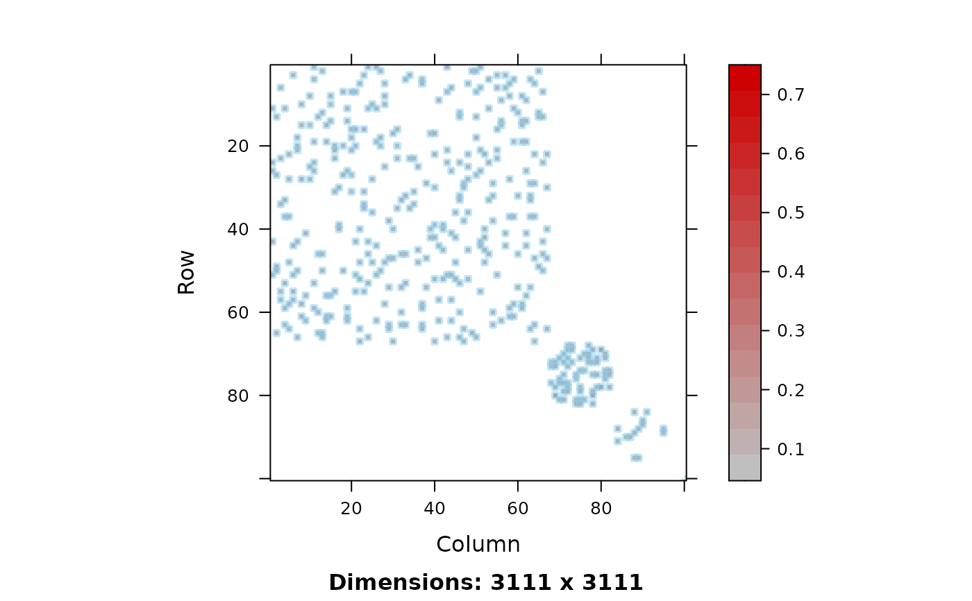
## using an opaque border color
image(USCounties, c(1,100), c(1,100), useAbs=FALSE, lwd=3, border.col = adjustcolor("skyblue", 1/2))
I2 <- image(USCounties, c(1,100), c(1,100), useAbs=FALSE, border.col=NA)
I3 <- image(USCounties, c(1,100), c(1,100), useAbs=FALSE, lwd=2, border.col=NA)
stopifnot(all.equal(I1, I2, check.environment=FALSE),
all.equal(I2, I3, check.environment=FALSE))
## using an opaque border color
image(USCounties, c(1,100), c(1,100), useAbs=FALSE, lwd=3, border.col = adjustcolor("skyblue", 1/2))
 if(interactive() || nzchar(Sys.getenv("R_MATRIX_CHECK_EXTRA"))) {
## Using raster graphics: For PDF this would give a 77 MB file,
## however, for such a large matrix, this is typically considerably
## *slower* (than vector graphics rectangles) in most cases :
if(doPNG <- !dev.interactive())
png("image-USCounties-raster.png", width=3200, height=3200)
image(USCounties, useRaster = TRUE) # should not suffer from anti-aliasing
if(doPNG)
dev.off()
## and now look at the *.png image in a viewer you can easily zoom in and out
}#only if(doExtras)
if(interactive() || nzchar(Sys.getenv("R_MATRIX_CHECK_EXTRA"))) {
## Using raster graphics: For PDF this would give a 77 MB file,
## however, for such a large matrix, this is typically considerably
## *slower* (than vector graphics rectangles) in most cases :
if(doPNG <- !dev.interactive())
png("image-USCounties-raster.png", width=3200, height=3200)
image(USCounties, useRaster = TRUE) # should not suffer from anti-aliasing
if(doPNG)
dev.off()
## and now look at the *.png image in a viewer you can easily zoom in and out
}#only if(doExtras)