Bootstrap Repeated Measurements Model
rm.boot.RdFor a dataset containing a time variable, a scalar response variable,
and an optional subject identification variable, obtains least squares
estimates of the coefficients of a restricted cubic spline function or
a linear regression in time after adjusting for subject effects
through the use of subject dummy variables. Then the fit is
bootstrapped B times, either by treating time and subject ID as
fixed (i.e., conditioning the analysis on them) or as random
variables. For the former, the residuals from the original model fit
are used as the basis of the bootstrap distribution. For the latter,
samples are taken jointly from the time, subject ID, and response
vectors to obtain unconditional distributions.
If a subject id variable is given, the bootstrap sampling will
be based on samples with replacement from subjects rather than from
individual data points. In other words, either none or all of a given
subject's data will appear in a bootstrap sample. This cluster
sampling takes into account any correlation structure that might exist
within subjects, so that confidence limits are corrected for
within-subject correlation. Assuming that ordinary least squares
estimates, which ignore the correlation structure, are consistent
(which is almost always true) and efficient (which would not be true
for certain correlation structures or for datasets in which the number
of observation times vary greatly from subject to subject), the
resulting analysis will be a robust, efficient repeated measures
analysis for the one-sample problem.
Predicted values of the fitted models are evaluated by default at a grid of 100 equally spaced time points ranging from the minimum to maximum observed time points. Predictions are for the average subject effect. Pointwise confidence intervals are optionally computed separately for each of the points on the time grid. However, simultaneous confidence regions that control the level of confidence for the entire regression curve lying within a band are often more appropriate, as they allow the analyst to draw conclusions about nuances in the mean time response profile that were not stated apriori. The method of Tibshirani (1997) is used to easily obtain simultaneous confidence sets for the set of coefficients of the spline or linear regression function as well as the average intercept parameter (over subjects). Here one computes the objective criterion (here both the -2 log likelihood evaluated at the bootstrap estimate of beta but with respect to the original design matrix and response vector, and the sum of squared errors in predicting the original response vector) for the original fit as well as for all of the bootstrap fits. The confidence set of the regression coefficients is the set of all coefficients that are associated with objective function values that are less than or equal to say the 0.95 quantile of the vector of \(\code{B} + 1\) objective function values. For the coefficients satisfying this condition, predicted curves are computed at the time grid, and minima and maxima of these curves are computed separately at each time point toderive the final simultaneous confidence band.
By default, the log likelihoods that are computed for obtaining the
simultaneous confidence band assume independence within subject. This
will cause problems unless such log likelihoods have very high rank
correlation with the log likelihood allowing for dependence. To allow
for correlation or to estimate the correlation function, see the
cor.pattern argument below.
Usage
rm.boot(time, y, id=seq(along=time), subset,
        plot.individual=FALSE,
        bootstrap.type=c('x fixed','x random'),
        nk=6, knots, B=500, smoother=supsmu,
        xlab, xlim, ylim=range(y),
        times=seq(min(time), max(time), length=100),
        absorb.subject.effects=FALSE,
        rho=0, cor.pattern=c('independent','estimate'), ncor=10000,
        ...)


# S3 method for class 'rm.boot'
plot(x, obj2, conf.int=.95,
     xlab=x$xlab, ylab=x$ylab,
     xlim, ylim=x$ylim,
     individual.boot=FALSE,
     pointwise.band=FALSE,
     curves.in.simultaneous.band=FALSE,
     col.pointwise.band=2,
     objective=c('-2 log L','sse','dep -2 log L'), add=FALSE, ncurves,
     multi=FALSE, multi.method=c('color','density'),
     multi.conf   =c(.05,.1,.2,.3,.4,.5,.6,.7,.8,.9,.95,.99),
     multi.density=c( -1,90,80,70,60,50,40,30,20,10,  7,  4),
     multi.col    =c(  1, 8,20, 5, 2, 7,15,13,10,11,  9, 14),
     subtitles=TRUE, ...)
Arguments
- time
numeric time vector
- y
continuous numeric response vector of length the same as
time. Subjects having multiple measurements have the measurements strung out.- x
an object returned from
rm.boot- id
subject ID variable. If omitted, it is assumed that each time-response pair is measured on a different subject.
- subset
subset of observations to process if not all the data
- plot.individual
set to
TRUEto plot nonparametrically smoothed time-response curves for each subject- bootstrap.type
specifies whether to treat the time and subject ID variables as fixed or random
- nk
number of knots in the restricted cubic spline function fit. The number of knots may be 0 (denoting linear regression) or an integer greater than 2 in which k knots results in \(k - 1\) regression coefficients excluding the intercept. The default is 6 knots.
- knots
vector of knot locations. May be specified if
nkis omitted.- B
number of bootstrap repetitions. Default is 500.
- smoother
a smoothing function that is used if
plot.individual=TRUE. Default issupsmu.- xlab
label for x-axis. Default is
"units"attribute of the originaltimevariable, or"Time"if no such attribute was defined using theunitsfunction.- xlim
specifies x-axis plotting limits. Default is to use range of times specified to
rm.boot.- ylim
for
rm.bootthis is a vector of y-axis limits used ifplot.individual=TRUE. It is also passed along for later use byplot.rm.boot. Forplot.rm.boot,ylimcan be specified, to override the value stored in the object stored byrm.boot. The default is the actual range ofyin the input data.- times
a sequence of times at which to evaluated fitted values and confidence limits. Default is 100 equally spaced points in the observed range of
time.- absorb.subject.effects
If
TRUE, adjusts the response vectorybefore re-sampling so that the subject-specific effects in the initial model fit are all zero. Then in re-sampling, subject effects are not used in the models. This will downplay one of the sources of variation. This option is used mainly for checking for consistency of results, as the re-sampling analyses are simpler whenabsort.subject.effects=TRUE.- rho
The log-likelihood function that is used as the basis of simultaneous confidence bands assumes normality with independence within subject. To check the robustness of this assumption, if
rhois not zero, the log-likelihood under multivariate normality within subject, with constant correlationrhobetween any two time points, is also computed. If the two log-likelihoods have the same ranks across re-samples, alllowing the correlation structure does not matter. The agreement in ranks is quantified using the Spearman rank correlation coefficient. Theplotmethod allows the non-zero intra-subject correlation log-likelihood to be used in deriving the simultaneous confidence band. Note that this approach does assume homoscedasticity.- cor.pattern
More generally than using an equal-correlation structure, you can specify a function of two time vectors that generates as many correlations as the length of these vectors. For example,
cor.pattern=function(time1,time2) 0.2^(abs(time1-time2)/10)would specify a dampening serial correlation pattern.cor.patterncan also be a list containing vectorsx(a vector of absolute time differences) andy(a corresponding vector of correlations). To estimate the correlation function as a function of absolute time differences within subjects, specifycor.pattern="estimate". The products of all possible pairs of residuals (or at least up toncorof them) within subjects will be related to the absolute time difference. The correlation function is estimated by computing the sample mean of the products of standardized residuals, stratified by absolute time difference. The correlation for a zero time difference is set to 1 regardless of thelowessestimate. NOTE: This approach fails in the presence of large subject effects; correcting for such effects removes too much of the correlation structure in the residuals.- ncor
the maximum number of pairs of time values used in estimating the correlation function if
cor.pattern="estimate"- ...
other arguments to pass to
smootherifplot.individual=TRUE- obj2
a second object created by
rm.bootthat can also be passed toplot.rm.boot. This is used for two-sample problems for which the time profiles are allowed to differ between the two groups. The bootstrapped predicted y values for the second fit are subtracted from the fitted values for the first fit so that the predicted mean response for group 1 minus the predicted mean response for group 2 is what is plotted. The confidence bands that are plotted are also for this difference. For the simultaneous confidence band, the objective criterion is taken to be the sum of the objective criteria (-2 log L or sum of squared errors) for the separate fits for the two groups. Thetimesvectors must have been identical for both calls torm.boot, althoughNAs can be inserted by the user of one or both of the time vectors in therm.bootobjects so as to suppress certain sections of the difference curve from being plotted.- conf.int
the confidence level to use in constructing simultaneous, and optionally pointwise, bands. Default is 0.95.
- ylab
label for y-axis. Default is the
"label"attribute of the originalyvariable, or"y"if no label was assigned toy(using thelabelfunction, for example).- individual.boot
set to
TRUEto plot the first 100 bootstrap regression fits- pointwise.band
set to
TRUEto draw a pointwise confidence band in addition to the simultaneous band- curves.in.simultaneous.band
set to
TRUEto draw all bootstrap regression fits that had a sum of squared errors (obtained by predicting the originalyvector from the originaltimevector andidvector) that was less that or equal to theconf.intquantile of all bootstrapped models (plus the original model). This will show how the point by point max and min were computed to form the simultaneous confidence band.- col.pointwise.band
color for the pointwise confidence band. Default is 2, which defaults to red for default Windows S-PLUS setups.
- objective
the default is to use the -2 times log of the Gaussian likelihood for computing the simultaneous confidence region. If neither
cor.patternnorrhowas specified torm.boot, the independent homoscedastic Gaussian likelihood is used. Otherwise the dependent homoscedastic likelihood is used according to the specified or estimated correlation pattern. Specifyobjective="sse"to instead use the sum of squared errors.- add
set to
TRUEto add curves to an existing plot. If you do this, titles and subtitles are omitted.- ncurves
when using
individual.boot=TRUEorcurves.in.simultaneous.band=TRUE, you can plot a random sample ofncurvesof the fitted curves instead of plotting up toBof them.- multi
set to
TRUEto draw multiple simultaneous confidence bands shaded with different colors. Confidence levels vary over the values in themulti.confvector.- multi.method
specifies the method of shading when
multi=TRUE. Default is to use colors, with the default colors chosen so that when the graph is printed under S-Plus for Windows 4.0 to an HP LaserJet printer, the confidence regions are naturally ordered by darkness of gray-scale. Regions closer to the point estimates (i.e., the center) are darker. Specifymulti.method="density"to instead use densities of lines drawn per inch in the confidence regions, with all regions drawn with the default color. Thepolygonfunction is used to shade the regions.- multi.conf
vector of confidence levels, in ascending order. Default is to use 12 confidence levels ranging from 0.05 to 0.99.
- multi.density
vector of densities in lines per inch corresponding to
multi.conf. As is the convention in thepolygonfunction, a density of -1 indicates a solid region.- multi.col
vector of colors corresponding to
multi.conf. Seemulti.methodfor rationale.- subtitles
set to
FALSEto suppress drawing subtitles for the plot
Value
an object of class rm.boot is returned by rm.boot. The
principal object stored in the returned object is a matrix of
regression coefficients for the original fit and all of the bootstrap
repetitions (object Coef), along with vectors of the
corresponding -2 log likelihoods are sums of squared errors. The
original fit object from lm.fit.qr is stored in
fit. For this fit, a cell means model is used for the
id effects.
plot.rm.boot returns a list containing the vector of times used
for plotting along with the overall fitted values, lower and upper
simultaneous confidence limits, and optionally the pointwise
confidence limits.
Details
Observations having missing time or y are excluded from
the analysis.
As most repeated measurement studies consider the times as design
points, the fixed covariable case is the default. Bootstrapping the
residuals from the initial fit assumes that the model is correctly
specified. Even if the covariables are fixed, doing an unconditional
bootstrap is still appropriate, and for large sample sizes
unconditional confidence intervals are only slightly wider than
conditional ones. For moderate to small sample sizes, the
bootstrap.type="x random" method can be fairly conservative.
If not all subjects have the same number of observations (after
deleting observations containing missing values) and if
bootstrap.type="x fixed", bootstrapped residual vectors may
have a length m that is different from the number of original
observations n. If \(m > n\) for a bootstrap
repetition, the first n elements of the randomly drawn residuals
are used. If \(m < n\), the residual vector is appended
with a random sample with replacement of length \(n - m\) from itself. A warning message is issued if this happens.
If the number of time points per subject varies, the bootstrap results
for bootstrap.type="x fixed" can still be invalid, as this
method assumes that a vector (over subjects) of all residuals can be
added to the original yhats, and varying number of points will cause
mis-alignment.
For bootstrap.type="x random" in the presence of significant
subject effects, the analysis is approximate as the subjects used in
any one bootstrap fit will not be the entire list of subjects. The
average (over subjects used in the bootstrap sample) intercept is used
from that bootstrap sample as a predictor of average subject effects
in the overall sample.
Once the bootstrap coefficient matrix is stored by rm.boot,
plot.rm.boot can be run multiple times with different options
(e.g, different confidence levels).
See bootcov in the rms library for a general
approach to handling repeated measurement data for ordinary linear
models, binary and ordinal models, and survival models, using the
unconditional bootstrap. bootcov does not handle bootstrapping
residuals.
Author
Frank Harrell
Department of Biostatistics
Vanderbilt University School of Medicine
fh@fharrell.com
References
Feng Z, McLerran D, Grizzle J (1996): A comparison of statistical methods for clustered data analysis with Gaussian error. Stat in Med 15:1793–1806.
Tibshirani R, Knight K (1997):Model search and inference by bootstrap
"bumping". Technical Report, Department of Statistics, University of Toronto.
https://www.jstor.org/stable/1390820. Presented at the Joint Statistical
Meetings, Chicago, August 1996.
Efron B, Tibshirani R (1993): An Introduction to the Bootstrap. New York: Chapman and Hall.
Diggle PJ, Verbyla AP (1998): Nonparametric estimation of covariance structure in logitudinal data. Biometrics 54:401–415.
Chapman IM, Hartman ML, et al (1997): Effect of aging on the sensitivity of growth hormone secretion to insulin-like growth factor-I negative feedback. J Clin Endocrinol Metab 82:2996–3004.
Li Y, Wang YG (2008): Smooth bootstrap methods for analysis of longitudinal data. Stat in Med 27:937-953. (potential improvements to cluster bootstrap; not implemented here)
Examples
# Generate multivariate normal responses with equal correlations (.7)
# within subjects and no correlation between subjects
# Simulate realizations from a piecewise linear population time-response
# profile with large subject effects, and fit using a 6-knot spline
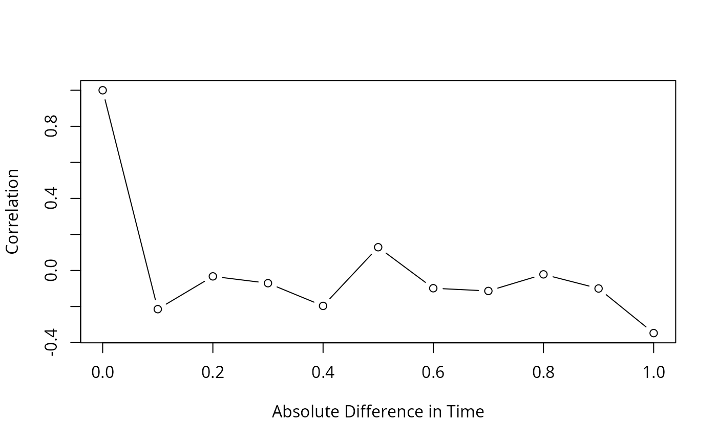
# Estimate the correlation structure from the residuals, as a function
# of the absolute time difference
# Function to generate n p-variate normal variates with mean vector u and
# covariance matrix S
# Slight modification of function written by Bill Venables
# See also the built-in function rmvnorm
mvrnorm <- function(n, p = 1, u = rep(0, p), S = diag(p)) {
Z <- matrix(rnorm(n * p), p, n)
t(u + t(chol(S)) %*% Z)
}
n <- 20 # Number of subjects
sub <- .5*(1:n) # Subject effects
# Specify functional form for time trend and compute non-stochastic component
times <- seq(0, 1, by=.1)
g <- function(times) 5*pmax(abs(times-.5),.3)
ey <- g(times)
# Generate multivariate normal errors for 20 subjects at 11 times
# Assume equal correlations of rho=.7, independent subjects
nt <- length(times)
rho <- .7
set.seed(19)
errors <- mvrnorm(n, p=nt, S=diag(rep(1-rho,nt))+rho)
# Note: first random number seed used gave rise to mean(errors)=0.24!
# Add E[Y], error components, and subject effects
y <- matrix(rep(ey,n), ncol=nt, byrow=TRUE) + errors +
matrix(rep(sub,nt), ncol=nt)
# String out data into long vectors for times, responses, and subject ID
y <- as.vector(t(y))
times <- rep(times, n)
id <- sort(rep(1:n, nt))
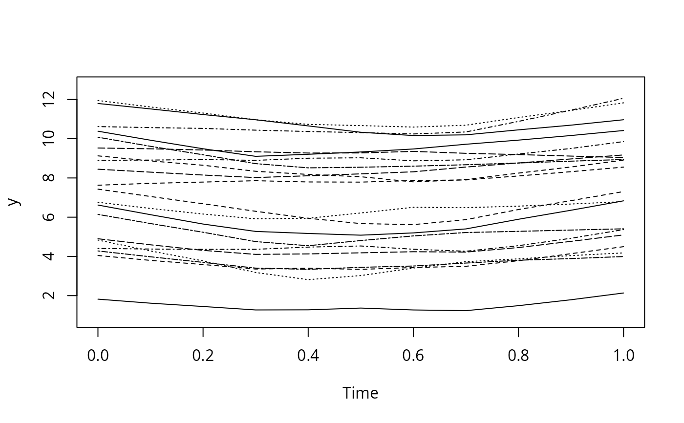
# Show lowess estimates of time profiles for individual subjects
f <- rm.boot(times, y, id, plot.individual=TRUE, B=25, cor.pattern='estimate',
smoother=lowess, bootstrap.type='x fixed', nk=6)
 #> 10 20
#>
#> Spearman rank correlation between 26 log likelihoods assuming independence and assuming dependence: 0.95
# In practice use B=400 or 500
# This will compute a dependent-structure log-likelihood in addition
# to one assuming independence. By default, the dep. structure
# objective will be used by the plot method (could have specified rho=.7)
# NOTE: Estimating the correlation pattern from the residual does not
# work in cases such as this one where there are large subject effects
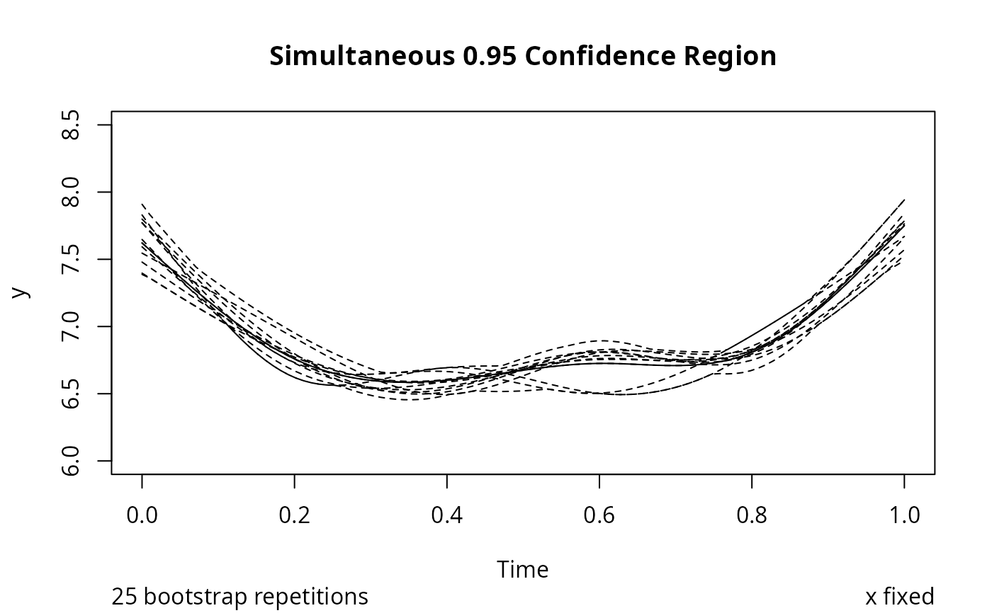
# Plot fits for a random sample of 10 of the 25 bootstrap fits
plot(f, individual.boot=TRUE, ncurves=10, ylim=c(6,8.5))
#> 10 20
#>
#> Spearman rank correlation between 26 log likelihoods assuming independence and assuming dependence: 0.95
# In practice use B=400 or 500
# This will compute a dependent-structure log-likelihood in addition
# to one assuming independence. By default, the dep. structure
# objective will be used by the plot method (could have specified rho=.7)
# NOTE: Estimating the correlation pattern from the residual does not
# work in cases such as this one where there are large subject effects
# Plot fits for a random sample of 10 of the 25 bootstrap fits
plot(f, individual.boot=TRUE, ncurves=10, ylim=c(6,8.5))
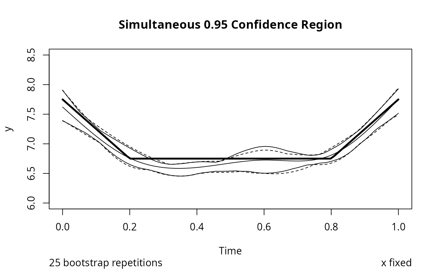
 # Plot pointwise and simultaneous confidence regions
plot(f, pointwise.band=TRUE, col.pointwise=1, ylim=c(6,8.5))
# Plot population response curve at average subject effect
ts <- seq(0, 1, length=100)
lines(ts, g(ts)+mean(sub), lwd=3)
# Plot pointwise and simultaneous confidence regions
plot(f, pointwise.band=TRUE, col.pointwise=1, ylim=c(6,8.5))
# Plot population response curve at average subject effect
ts <- seq(0, 1, length=100)
lines(ts, g(ts)+mean(sub), lwd=3)
 if (FALSE) { # \dontrun{
#
# Handle a 2-sample problem in which curves are fitted
# separately for males and females and we wish to estimate the
# difference in the time-response curves for the two sexes.
# The objective criterion will be taken by plot.rm.boot as the
# total of the two sums of squared errors for the two models
#
knots <- rcspline.eval(c(time.f,time.m), nk=6, knots.only=TRUE)
# Use same knots for both sexes, and use a times vector that
# uses a range of times that is included in the measurement
# times for both sexes
#
tm <- seq(max(min(time.f),min(time.m)),
min(max(time.f),max(time.m)),length=100)
f.female <- rm.boot(time.f, bp.f, id.f, knots=knots, times=tm)
f.male <- rm.boot(time.m, bp.m, id.m, knots=knots, times=tm)
plot(f.female)
plot(f.male)
# The following plots female minus male response, with
# a sequence of shaded confidence band for the difference
plot(f.female,f.male,multi=TRUE)
# Do 1000 simulated analyses to check simultaneous coverage
# probability. Use a null regression model with Gaussian errors
n.per.pt <- 30
n.pt <- 10
null.in.region <- 0
for(i in 1:1000) {
y <- rnorm(n.pt*n.per.pt)
time <- rep(1:n.per.pt, n.pt)
# Add the following line and add ,id=id to rm.boot to use clustering
# id <- sort(rep(1:n.pt, n.per.pt))
# Because we are ignoring patient id, this simulation is effectively
# using 1 point from each of 300 patients, with times 1,2,3,,,30
f <- rm.boot(time, y, B=500, nk=5, bootstrap.type='x fixed')
g <- plot(f, ylim=c(-1,1), pointwise=FALSE)
null.in.region <- null.in.region + all(g$lower<=0 & g$upper>=0)
prn(c(i=i,null.in.region=null.in.region))
}
# Simulation Results: 905/1000 simultaneous confidence bands
# fully contained the horizontal line at zero
} # }
if (FALSE) { # \dontrun{
#
# Handle a 2-sample problem in which curves are fitted
# separately for males and females and we wish to estimate the
# difference in the time-response curves for the two sexes.
# The objective criterion will be taken by plot.rm.boot as the
# total of the two sums of squared errors for the two models
#
knots <- rcspline.eval(c(time.f,time.m), nk=6, knots.only=TRUE)
# Use same knots for both sexes, and use a times vector that
# uses a range of times that is included in the measurement
# times for both sexes
#
tm <- seq(max(min(time.f),min(time.m)),
min(max(time.f),max(time.m)),length=100)
f.female <- rm.boot(time.f, bp.f, id.f, knots=knots, times=tm)
f.male <- rm.boot(time.m, bp.m, id.m, knots=knots, times=tm)
plot(f.female)
plot(f.male)
# The following plots female minus male response, with
# a sequence of shaded confidence band for the difference
plot(f.female,f.male,multi=TRUE)
# Do 1000 simulated analyses to check simultaneous coverage
# probability. Use a null regression model with Gaussian errors
n.per.pt <- 30
n.pt <- 10
null.in.region <- 0
for(i in 1:1000) {
y <- rnorm(n.pt*n.per.pt)
time <- rep(1:n.per.pt, n.pt)
# Add the following line and add ,id=id to rm.boot to use clustering
# id <- sort(rep(1:n.pt, n.per.pt))
# Because we are ignoring patient id, this simulation is effectively
# using 1 point from each of 300 patients, with times 1,2,3,,,30
f <- rm.boot(time, y, B=500, nk=5, bootstrap.type='x fixed')
g <- plot(f, ylim=c(-1,1), pointwise=FALSE)
null.in.region <- null.in.region + all(g$lower<=0 & g$upper>=0)
prn(c(i=i,null.in.region=null.in.region))
}
# Simulation Results: 905/1000 simultaneous confidence bands
# fully contained the horizontal line at zero
} # }