Re-state Restricted Cubic Spline Function

This function re-states a restricted cubic spline function in the un-linearly-restricted form. Coefficients for that form are returned, along with an R functional representation of this function and a LaTeX character representation of the function. rcsplineFunction is a fast function that creates a function to compute a restricted cubic spline function with given coefficients and knots, without reformatting the function to be pretty (i.e., into unrestricted form).

Usage

rcspline.restate(knots, coef,
                 type=c("ordinary","integral"),
                 x="X", lx=nchar(x),
                 norm=2, columns=65, before="& &", after="\\",
                 begin="", nbegin=0, digits=max(8, .Options$digits))

rcsplineFunction(knots, coef, norm=2, type=c('ordinary', 'integral'))

Arguments

knots: vector of knots used in the regression fit
coef: vector of coefficients from the fit. If the length of coef is \(k-1\), where k is equal to the length(knots), the first coefficient must be for the linear term and remaining \(k-2\) coefficients must be for the constructed terms (e.g., from rcspline.eval). If the length of coef is k, an intercept is assumed to be in the first element (or a zero is prepended to coef for rcsplineFunction).
type: The default is to represent the cubic spline function corresponding to the coefficients and knots. Set type = "integral" to instead represent its anti-derivative.
x: a character string to use as the variable name in the LaTeX expression for the formula.
lx: length of x to count with respect to columns. Default is length of character string contained by x. You may want to set lx smaller than this if it includes non-printable LaTeX commands.
norm: normalization that was used in deriving the original nonlinear terms used in the fit. See rcspline.eval for definitions.
columns: maximum number of symbols in the LaTeX expression to allow before inserting a newline (\\) command. Set to a very large number to keep text all on one line.
before: text to place before each line of LaTeX output. Use "& &" for an equation array environment in LaTeX where you want to have a left-hand prefix e.g. "f(X) & = &" or using "\lefteqn".
after: text to place at the end of each line of output.
begin: text with which to start the first line of output. Useful when adding LaTeX output to part of an existing formula
nbegin: number of columns of printable text in begin
digits: number of significant digits to write for coefficients and knots

Value

rcspline.restate returns a vector of coefficients. The coefficients are un-normalized and two coefficients are added that are linearly dependent on the other coefficients and knots. The vector of coefficients has four attributes. knots is a vector of knots, latex is a vector of text strings with the LaTeX representation of the formula. columns.used is the number of columns used in the output string since the last newline command. function is an R function, which is also return in character string format as the text attribute. rcsplineFunction returns an R function with arguments x (a user-supplied numeric vector at which to evaluate the function), and some automatically-supplied other arguments.

Author

Frank Harrell
Department of Biostatistics, Vanderbilt University
fh@fharrell.com

Examples

set.seed(1)
x <- 1:100
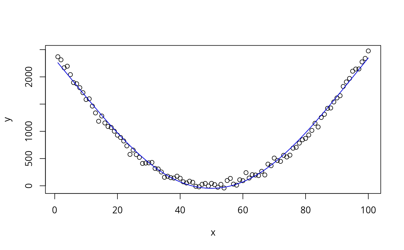
y <- (x - 50)^2 + rnorm(100, 0, 50)
plot(x, y)
xx <- rcspline.eval(x, inclx=TRUE, nk=4)
knots <- attr(xx, "knots")
coef <- lsfit(xx, y)$coef
options(digits=4)
# rcspline.restate must ignore intercept
w <- rcspline.restate(knots, coef[-1], x="{\\rm BP}")
# could also have used coef instead of coef[-1], to include intercept
cat(attr(w,"latex"), sep="\n")
#> & & -69.685564  {\rm BP}+0.013443742 ({\rm BP}-5.95)_{+}^{3} \
#> & & -0.013754656({\rm BP}-35.65)_{+}^{3}-0.012821915({\rm BP}-65.35)_{+}^{3} \
#> & & +0.013132828 ({\rm BP}-95.05)_{+}^{3} \


xtrans <- eval(attr(w, "function"))
# This is an S function of a single argument
lines(x, coef[1] + xtrans(x), type="l")
# Plots fitted transformation

xtrans <- rcsplineFunction(knots, coef)
xtrans
#> function (x = numeric(0), knots = c(5.95, 35.65, 65.35, 95.05
#> ), coef = c(Intercept = 2329.20175140574, x = -69.6855639459134, 
#> 106.727315060936, -109.195599900753), kd = 19.9488777705554, 
#>     type = "ordinary") 
#> {
#>     k <- length(knots)
#>     knotnk <- knots[k]
#>     knotnk1 <- knots[k - 1]
#>     knot1 <- knots[1]
#>     if (length(coef) < k) 
#>         coef <- c(0, coef)
#>     if (type == "ordinary") {
#>         y <- coef[1] + coef[2] * x
#>         for (j in 1:(k - 2)) y <- y + coef[j + 2] * (pmax((x - 
#>             knots[j])/kd, 0)^3 + ((knotnk1 - knots[j]) * pmax((x - 
#>             knotnk)/kd, 0)^3 - (knotnk - knots[j]) * (pmax((x - 
#>             knotnk1)/kd, 0)^3))/(knotnk - knotnk1))
#>         return(y)
#>     }
#>     y <- coef[1] * x + 0.5 * coef[2] * x * x
#>     for (j in 1:(k - 2)) y <- y + 0.25 * coef[j + 2] * kd * (pmax((x - 
#>         knots[j])/kd, 0)^4 + ((knotnk1 - knots[j]) * pmax((x - 
#>         knotnk)/kd, 0)^4 - (knotnk - knots[j]) * (pmax((x - knotnk1)/kd, 
#>         0)^4))/(knotnk - knotnk1))
#>     y
#> }
#> <environment: 0x5e2f8b148688>
lines(x, xtrans(x), col='blue')



#x <- blood.pressure
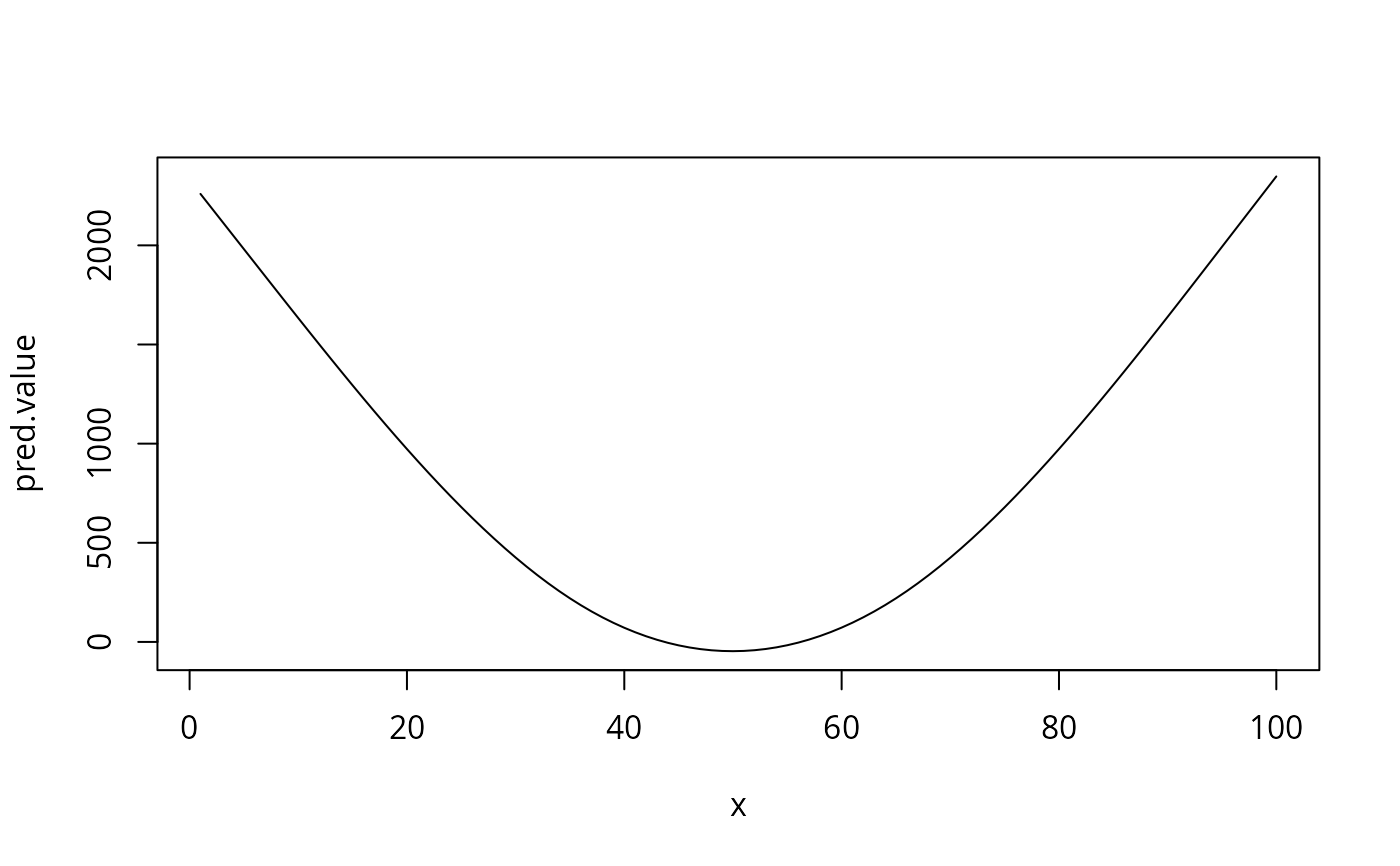
xx.simple <- cbind(x, pmax(x-knots[1],0)^3, pmax(x-knots[2],0)^3,
                       pmax(x-knots[3],0)^3, pmax(x-knots[4],0)^3)
pred.value <- coef[1] + xx.simple %*% w
plot(x, pred.value, type='l')   # same as above

Usage

Arguments

Value

Author

See also

Examples