Produces event.history graph for survival data
event.history.RdProduces an event history graph for right-censored survival data, including time-dependent covariate status, as described in Dubin, Muller, and Wang (2001). Effectively, a Kaplan-Meier curve is produced with supplementary information regarding individual survival information, censoring information, and status over time of an individual time-dependent covariate or time-dependent covariate function for both uncensored and censored individuals.
Usage
event.history(data, survtime.col, surv.col,
              surv.ind = c(1, 0), subset.rows = NULL,
              covtime.cols = NULL, cov.cols = NULL,
              num.colors = 1, cut.cov = NULL, colors = 1,
              cens.density = 10, mult.end.cens = 1.05,
              cens.mark.right =FALSE, cens.mark = "-",
              cens.mark.ahead = 0.5, cens.mark.cutoff = -1e-08,
              cens.mark.cex = 1,
              x.lab = "time under observation",
              y.lab = "estimated survival probability",
              title = "event history graph", ...)
Arguments
- data
A matrix or data frame with rows corresponding to units (often individuals) and columns corresponding to survival time, event/censoring indicator. Also, multiple columns may be devoted to time-dependent covariate level and time change.
- survtime.col
Column (in data) representing minimum of time-to-event or right-censoring time for individual.
- surv.col
Column (in data) representing event indicator for an individual. Though, traditionally, such an indicator will be 1 for an event and 0 for a censored observation, this indicator can be represented by any two numbers, made explicit by the surv.ind argument.
- surv.ind
Two-element vector representing, respectively, the number for an event, as listed in
surv.col, followed by the number for a censored observation. Default is traditional survival data represention, i.e.,c(1,0).- subset.rows
Subset of rows of original matrix or data frame (data) to place in event history graph. Logical arguments may be used here (e.g.,
treatment.arm == "a", if the data frame, data, has been attached to the search directory;- covtime.cols
Column(s) (in data) representing the time when change of time-dependent covariate (or time-dependent covariate function) occurs. There should be a unique non-
NAentry in the column for each such change (along with correspondingcov.colscolumn entry representing the value of the covariate or function at that change time). Default isNULL, meaning no time-dependent covariate information will be presented in the graph.- cov.cols
Column(s) (in data) representing the level of the time-dependent covariate (or time-dependent covariate function). There should be a unique non-
NAcolumn entry representing each change in the level (along with a corresponding covtime.cols column entry representing the time of the change). Default isNULL, meaning no time-dependent covariate information will be presented in the graph.- num.colors
Colors are utilized for the time-dependent covariate level for an individual. This argument provides the number of unique covariate levels which will be displayed by mapping the number of colors (via
num.colors) to the number of desired covariate levels. This will divide the covariate span into roughly equally-sized intervals, via the S-Plus cut function. Default is one color, meaning no time-dependent information will be presented in the graph. Note that this argument will be ignored/superceded if a non-NULL argument is provided for thecut.covparameter.- cut.cov
This argument allows the user to explicitly state how to define the intervals for the time-dependent covariate, such that different colors will be allocated to the user-defined covariate levels. For example, for plotting five colors, six ordered points within the span of the data's covariate levels should be provided. Default is
NULL, meaning that thenum.colorsargument value will dictate the number of breakpoints, with the covariate span defined into roughly equally-sized intervals via the S-Plus cut function. However, ifis.null(cut.cov) == FALSE, then this argument supercedes any entry for thenum.colorsargument.- colors
This is a vector argument defining the actual colors used for the time-dependent covariate levels in the plot, with the index of this vector corresponding to the ordered levels of the covariate. The number of colors (i.e., the length of the colors vector) should correspond to the value provided to the
num.colorsargument or the number of ordered points - 1 as defined in thecut.covargument (withcut.covsupercedingnum.colorsifis.null(cut.cov) == FALSE). The function, as currently written, allows for as much as twenty distinct colors. This argument effectively feeds into the col argument for the S-Plus polygon function. Default iscolors = 1. See the col argument for the both the S-Plus par function and polygon function for more information.- cens.density
This will provide the shading density at the end of the individual bars for those who are censored. For more information on shading density, see the density argument in the S-Plus polygon function. Default is
cens.density=10.- mult.end.cens
This is a multiplier that extends the length of the longest surviving individual bar (or bars, if a tie exists) if right-censored, presuming that no event times eventually follow this final censored time. Default extends the length 5 percent beyond the length of the observed right-censored survival time.
- cens.mark.right
A logical argument that states whether an explicit mark should be placed to the right of the individual right-censored survival bars. This argument is most useful for large sample sizes, where it may be hard to detect the special shading via cens.density, particularly for the short-term survivors.
- cens.mark
Character argument which describes the censored mark that should be used if
cens.mark.right = TRUE. Default is"-".- cens.mark.ahead
A numeric argument, which specifies the absolute distance to be placed between the individual right-censored survival bars and the mark as defined in the above cens.mark argument. Default is 0.5 (that is, a half of day, if survival time is measured in days), but may very well need adjusting depending on the maximum survival time observed in the dataset.
- cens.mark.cutoff
A negative number very close to 0 (by default
cens.mark.cutoff = -1e-8) to ensure that the censoring marks get plotted correctly. Seeevent.historycode in order to see its usage. This argument typically will not need adjustment.- cens.mark.cex
Numeric argument defining the size of the mark defined in the
cens.markargument above. See more information by viewing thecexargument for the S-Plusparfunction. Default iscens.mark.cex = 1.0.- x.lab
Single label to be used for entire x-axis. Default is
"time under observation".- y.lab
Single label to be used for entire y-axis. Default is
"estimated survival probability".- title
Title for the event history graph. Default is
"event history graph".- ...
This allows arguments to the plot function call within the
event.historyfunction. So, for example, the axes representations can be manipulated with appropriate arguments, or particular areas of theevent.historygraph can be “zoomed”. See the details section for more comments about zooming.
Details
In order to focus on a particular area of the event history graph,
zooming can be performed. This is best done by
specifying appropriate xlim and ylim
arguments at the end of the event.history function call,
taking advantage of the ... argument link to the plot function.
An example of zooming can be seen
in Plate 4 of the paper referenced below.
Please read the reference below to understand how the individual covariate and survival information is provided in the plot, how ties are handled, how right-censoring is handled, etc.
References
Dubin, J.A., Muller, H.-G., and Wang, J.-L. (2001). Event history graphs for censored survival data. Statistics in Medicine, 20, 2951-2964.
Author
Joel Dubin
jdubin@uwaterloo.ca
Note
The authors have found better control of the use of color by producing the graphs via the postscript plotting device in S-Plus. In fact, the provided examples utilize the postscript function. However, your past experiences may be different, and you may prefer to control color directly (to the graphsheet in Windows environment, for example). The event.history function will work with either approach.
WARNING
This function has been tested thoroughly, but only within a restricted version and environment, i.e., only within S-Plus 2000, Version 3, and within S-Plus 6.0, version 2, both on a Windows 2000 machine. Hence, we cannot currently vouch for the function's effectiveness in other versions of S-Plus (e.g., S-Plus 3.4) nor in other operating environments (e.g., Windows 95, Linux or Unix). The function has also been verified to work on R under Linux.
Examples
# Code to produce event history graphs for SIM paper
#
# before generating plots, some pre-processing needs to be performed,
# in order to get dataset in proper form for event.history function;
# need to create one line per subject and sort by time under observation,
# with those experiencing event coming before those tied with censoring time;
require('survival')
data(heart)
# creation of event.history version of heart dataset (call heart.one):
heart.one <- matrix(nrow=length(unique(heart$id)), ncol=8)
for(i in 1:length(unique(heart$id)))
{
if(length(heart$id[heart$id==i]) == 1)
heart.one[i,] <- as.numeric(unlist(heart[heart$id==i, ]))
else if(length(heart$id[heart$id==i]) == 2)
heart.one[i,] <- as.numeric(unlist(heart[heart$id==i,][2,]))
}
heart.one[,3][heart.one[,3] == 0] <- 2 ## converting censored events to 2, from 0
if(is.factor(heart$transplant))
heart.one[,7] <- heart.one[,7] - 1
## getting back to correct transplantation coding
heart.one <- as.data.frame(heart.one[order(unlist(heart.one[,2]), unlist(heart.one[,3])),])
names(heart.one) <- names(heart)
# back to usual censoring indicator:
heart.one[,3][heart.one[,3] == 2] <- 0
# note: transplant says 0 (for no transplants) or 1 (for one transplant)
# and event = 1 is death, while event = 0 is censored
# plot single Kaplan-Meier curve from heart data, first creating survival object
heart.surv <- survfit(Surv(stop, event) ~ 1, data=heart.one, conf.int = FALSE)
# figure 3: traditional Kaplan-Meier curve
# postscript('ehgfig3.ps', horiz=TRUE)
# omi <- par(omi=c(0,1.25,0.5,1.25))
plot(heart.surv, ylab='estimated survival probability',
xlab='observation time (in days)')
title('Figure 3: Kaplan-Meier curve for Stanford data', cex=0.8)
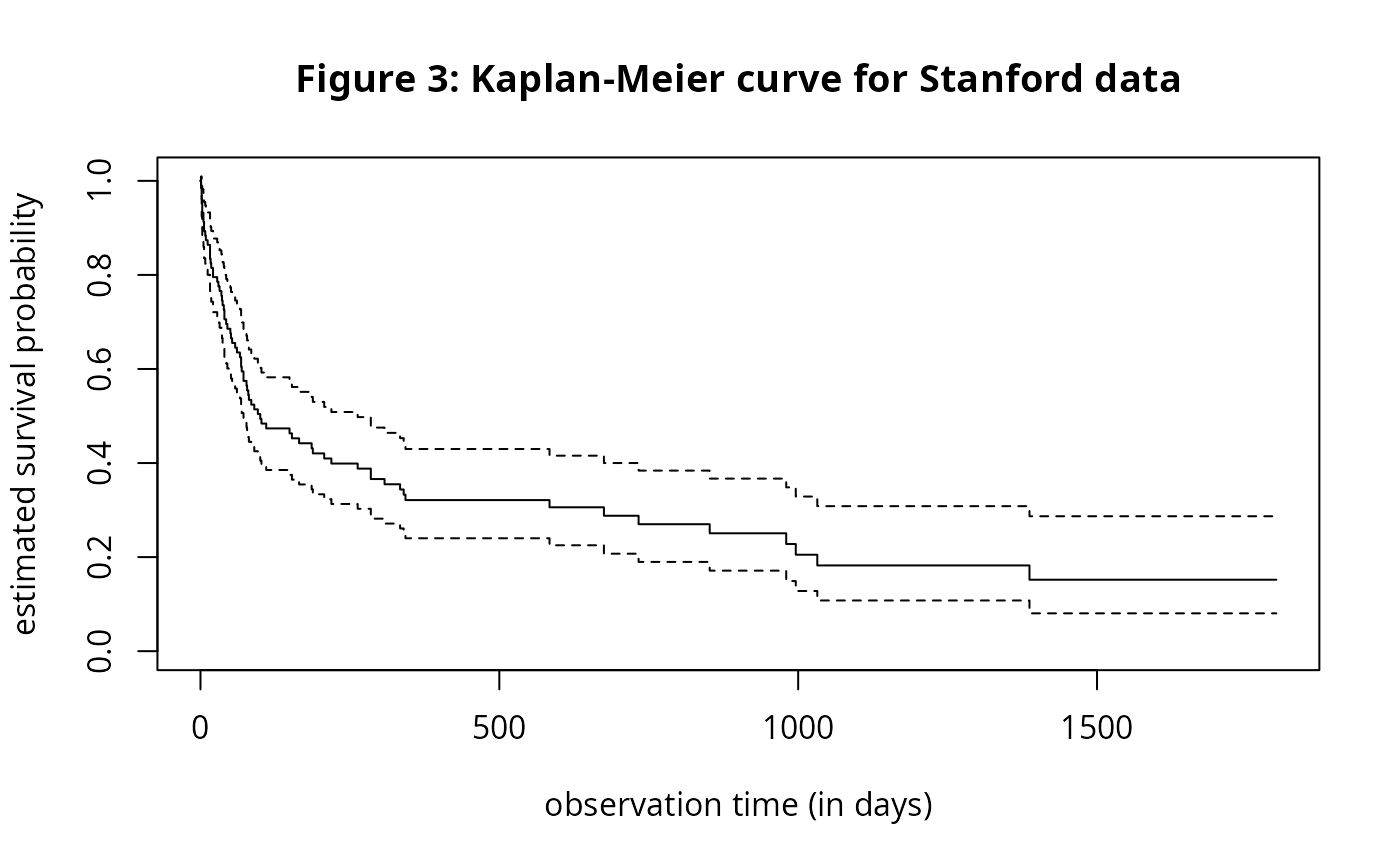 # dev.off()
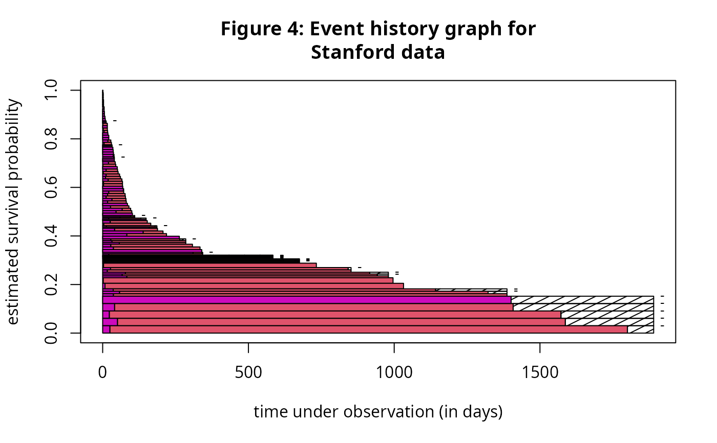
## now, draw event history graph for Stanford heart data; use as Figure 4
# postscript('ehgfig4.ps', horiz=TRUE, colors = seq(0, 1, len=20))
# par(omi=c(0,1.25,0.5,1.25))
event.history(heart.one,
survtime.col=heart.one[,2], surv.col=heart.one[,3],
covtime.cols = cbind(rep(0, dim(heart.one)[1]), heart.one[,1]),
cov.cols = cbind(rep(0, dim(heart.one)[1]), heart.one[,7]),
num.colors=2, colors=c(6,10),
x.lab = 'time under observation (in days)',
title='Figure 4: Event history graph for\nStanford data',
cens.mark.right =TRUE, cens.mark = '-',
cens.mark.ahead = 30.0, cens.mark.cex = 0.85)
# dev.off()
## now, draw event history graph for Stanford heart data; use as Figure 4
# postscript('ehgfig4.ps', horiz=TRUE, colors = seq(0, 1, len=20))
# par(omi=c(0,1.25,0.5,1.25))
event.history(heart.one,
survtime.col=heart.one[,2], surv.col=heart.one[,3],
covtime.cols = cbind(rep(0, dim(heart.one)[1]), heart.one[,1]),
cov.cols = cbind(rep(0, dim(heart.one)[1]), heart.one[,7]),
num.colors=2, colors=c(6,10),
x.lab = 'time under observation (in days)',
title='Figure 4: Event history graph for\nStanford data',
cens.mark.right =TRUE, cens.mark = '-',
cens.mark.ahead = 30.0, cens.mark.cex = 0.85)
 # dev.off()
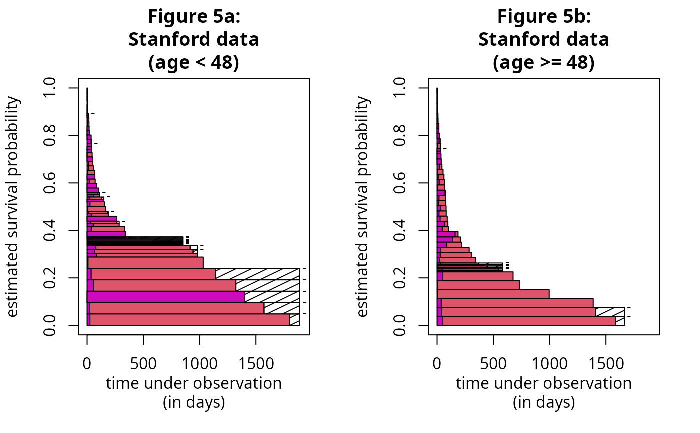
# now, draw age-stratified event history graph for Stanford heart data;
# use as Figure 5
# two plots, stratified by age status
# postscript('c:\temp\ehgfig5.ps', horiz=TRUE, colors = seq(0, 1, len=20))
# par(omi=c(0,1.25,0.5,1.25))
par(mfrow=c(1,2))
event.history(data=heart.one, subset.rows = (heart.one[,4] < 0),
survtime.col=heart.one[,2], surv.col=heart.one[,3],
covtime.cols = cbind(rep(0, dim(heart.one)[1]), heart.one[,1]),
cov.cols = cbind(rep(0, dim(heart.one)[1]), heart.one[,7]),
num.colors=2, colors=c(6,10),
x.lab = 'time under observation\n(in days)',
title = 'Figure 5a:\nStanford data\n(age < 48)',
cens.mark.right =TRUE, cens.mark = '-',
cens.mark.ahead = 40.0, cens.mark.cex = 0.85,
xlim=c(0,1900))
event.history(data=heart.one, subset.rows = (heart.one[,4] >= 0),
survtime.col=heart.one[,2], surv.col=heart.one[,3],
covtime.cols = cbind(rep(0, dim(heart.one)[1]), heart.one[,1]),
cov.cols = cbind(rep(0, dim(heart.one)[1]), heart.one[,7]),
num.colors=2, colors=c(6,10),
x.lab = 'time under observation\n(in days)',
title = 'Figure 5b:\nStanford data\n(age >= 48)',
cens.mark.right =TRUE, cens.mark = '-',
cens.mark.ahead = 40.0, cens.mark.cex = 0.85,
xlim=c(0,1900))
# dev.off()
# now, draw age-stratified event history graph for Stanford heart data;
# use as Figure 5
# two plots, stratified by age status
# postscript('c:\temp\ehgfig5.ps', horiz=TRUE, colors = seq(0, 1, len=20))
# par(omi=c(0,1.25,0.5,1.25))
par(mfrow=c(1,2))
event.history(data=heart.one, subset.rows = (heart.one[,4] < 0),
survtime.col=heart.one[,2], surv.col=heart.one[,3],
covtime.cols = cbind(rep(0, dim(heart.one)[1]), heart.one[,1]),
cov.cols = cbind(rep(0, dim(heart.one)[1]), heart.one[,7]),
num.colors=2, colors=c(6,10),
x.lab = 'time under observation\n(in days)',
title = 'Figure 5a:\nStanford data\n(age < 48)',
cens.mark.right =TRUE, cens.mark = '-',
cens.mark.ahead = 40.0, cens.mark.cex = 0.85,
xlim=c(0,1900))
event.history(data=heart.one, subset.rows = (heart.one[,4] >= 0),
survtime.col=heart.one[,2], surv.col=heart.one[,3],
covtime.cols = cbind(rep(0, dim(heart.one)[1]), heart.one[,1]),
cov.cols = cbind(rep(0, dim(heart.one)[1]), heart.one[,7]),
num.colors=2, colors=c(6,10),
x.lab = 'time under observation\n(in days)',
title = 'Figure 5b:\nStanford data\n(age >= 48)',
cens.mark.right =TRUE, cens.mark = '-',
cens.mark.ahead = 40.0, cens.mark.cex = 0.85,
xlim=c(0,1900))
 # dev.off()
# par(omi=omi)
# we will not show liver cirrhosis data manipulation, as it was
# a bit detailed; however, here is the
# event.history code to produce Figure 7 / Plate 1
# Figure 7 / Plate 1 : prothrombin ehg with color
if (FALSE) { # \dontrun{
second.arg <- 1 ### second.arg is for shading
third.arg <- c(rep(1,18),0,1) ### third.arg is for intensity
# postscript('c:\temp\ehgfig7.ps', horiz=TRUE,
# colors = cbind(seq(0, 1, len = 20), second.arg, third.arg))
# par(omi=c(0,1.25,0.5,1.25), col=19)
event.history(cirrhos2.eh, subset.rows = NULL,
survtime.col=cirrhos2.eh$time, surv.col=cirrhos2.eh$event,
covtime.cols = as.matrix(cirrhos2.eh[, ((2:18)*2)]),
cov.cols = as.matrix(cirrhos2.eh[, ((2:18)*2) + 1]),
cut.cov = as.numeric(quantile(as.matrix(cirrhos2.eh[, ((2:18)*2) + 1]),
c(0,.2,.4,.6,.8,1), na.rm=TRUE) + c(-1,0,0,0,0,1)),
colors=c(20,4,8,11,14),
x.lab = 'time under observation (in days)',
title='Figure 7: Event history graph for liver cirrhosis data (color)',
cens.mark.right =TRUE, cens.mark = '-',
cens.mark.ahead = 100.0, cens.mark.cex = 0.85)
# dev.off()
} # }
# dev.off()
# par(omi=omi)
# we will not show liver cirrhosis data manipulation, as it was
# a bit detailed; however, here is the
# event.history code to produce Figure 7 / Plate 1
# Figure 7 / Plate 1 : prothrombin ehg with color
if (FALSE) { # \dontrun{
second.arg <- 1 ### second.arg is for shading
third.arg <- c(rep(1,18),0,1) ### third.arg is for intensity
# postscript('c:\temp\ehgfig7.ps', horiz=TRUE,
# colors = cbind(seq(0, 1, len = 20), second.arg, third.arg))
# par(omi=c(0,1.25,0.5,1.25), col=19)
event.history(cirrhos2.eh, subset.rows = NULL,
survtime.col=cirrhos2.eh$time, surv.col=cirrhos2.eh$event,
covtime.cols = as.matrix(cirrhos2.eh[, ((2:18)*2)]),
cov.cols = as.matrix(cirrhos2.eh[, ((2:18)*2) + 1]),
cut.cov = as.numeric(quantile(as.matrix(cirrhos2.eh[, ((2:18)*2) + 1]),
c(0,.2,.4,.6,.8,1), na.rm=TRUE) + c(-1,0,0,0,0,1)),
colors=c(20,4,8,11,14),
x.lab = 'time under observation (in days)',
title='Figure 7: Event history graph for liver cirrhosis data (color)',
cens.mark.right =TRUE, cens.mark = '-',
cens.mark.ahead = 100.0, cens.mark.cex = 0.85)
# dev.off()
} # }