Data and Examples from Winkelmann and Boes (2009)
WinkelmannBoes2009.RdThis manual page collects a list of examples from the book. Some solutions might not be exact and the list is not complete. If you have suggestions for improvement (preferably in the form of code), please contact the package maintainer.
References
Winkelmann, R., and Boes, S. (2009). Analysis of Microdata, 2nd ed. Berlin and Heidelberg: Springer-Verlag.
Examples
#> Loading required namespace: ROCR
#> Loading required namespace: truncreg
# \donttest{
#########################################
## US General Social Survey 1974--2002 ##
#########################################
## data
data("GSS7402", package = "AER")
## completed fertility subset
gss40 <- subset(GSS7402, age >= 40)
## Chapter 1
## Table 1.1
gss_kids <- table(gss40$kids)
cbind(absolute = gss_kids,
relative = round(prop.table(gss_kids) * 100, digits = 2))
#> absolute relative
#> 0 744 14.45
#> 1 706 13.71
#> 2 1368 26.56
#> 3 1002 19.46
#> 4 593 11.51
#> 5 309 6.00
#> 6 190 3.69
#> 7 89 1.73
#> 8 149 2.89
## Table 1.2
sd1 <- function(x) sd(x) / sqrt(length(x))
with(gss40, round(cbind(
"obs" = tapply(kids, year, length),
"av kids" = tapply(kids, year, mean),
" " = tapply(kids, year, sd1),
"prop childless" = tapply(kids, year, function(x) mean(x <= 0)),
" " = tapply(kids, year, function(x) sd1(x <= 0)),
"av schooling" = tapply(education, year, mean),
" " = tapply(education, year, sd1)
), digits = 2))
#> obs av kids prop childless av schooling
#> 1974 410 3.17 0.10 0.09 0.01 11.07 0.16
#> 1978 445 2.73 0.09 0.14 0.02 11.00 0.15
#> 1982 577 2.96 0.09 0.14 0.01 11.05 0.14
#> 1986 470 2.70 0.09 0.16 0.02 11.34 0.14
#> 1990 431 2.50 0.08 0.15 0.02 12.41 0.15
#> 1994 989 2.40 0.06 0.15 0.01 12.78 0.10
#> 1998 911 2.42 0.06 0.15 0.01 12.94 0.11
#> 2002 917 2.36 0.06 0.16 0.01 13.25 0.10
## Table 1.3
gss40$trend <- gss40$year - 1974
kids_lm1 <- lm(kids ~ factor(year), data = gss40)
kids_lm2 <- lm(kids ~ trend, data = gss40)
kids_lm3 <- lm(kids ~ trend + education, data = gss40)
## Chapter 2
## Table 2.1
kids_tab <- prop.table(xtabs(~ kids + year, data = gss40), 2) * 100
round(kids_tab[,c(4, 8)], digits = 2)
#> year
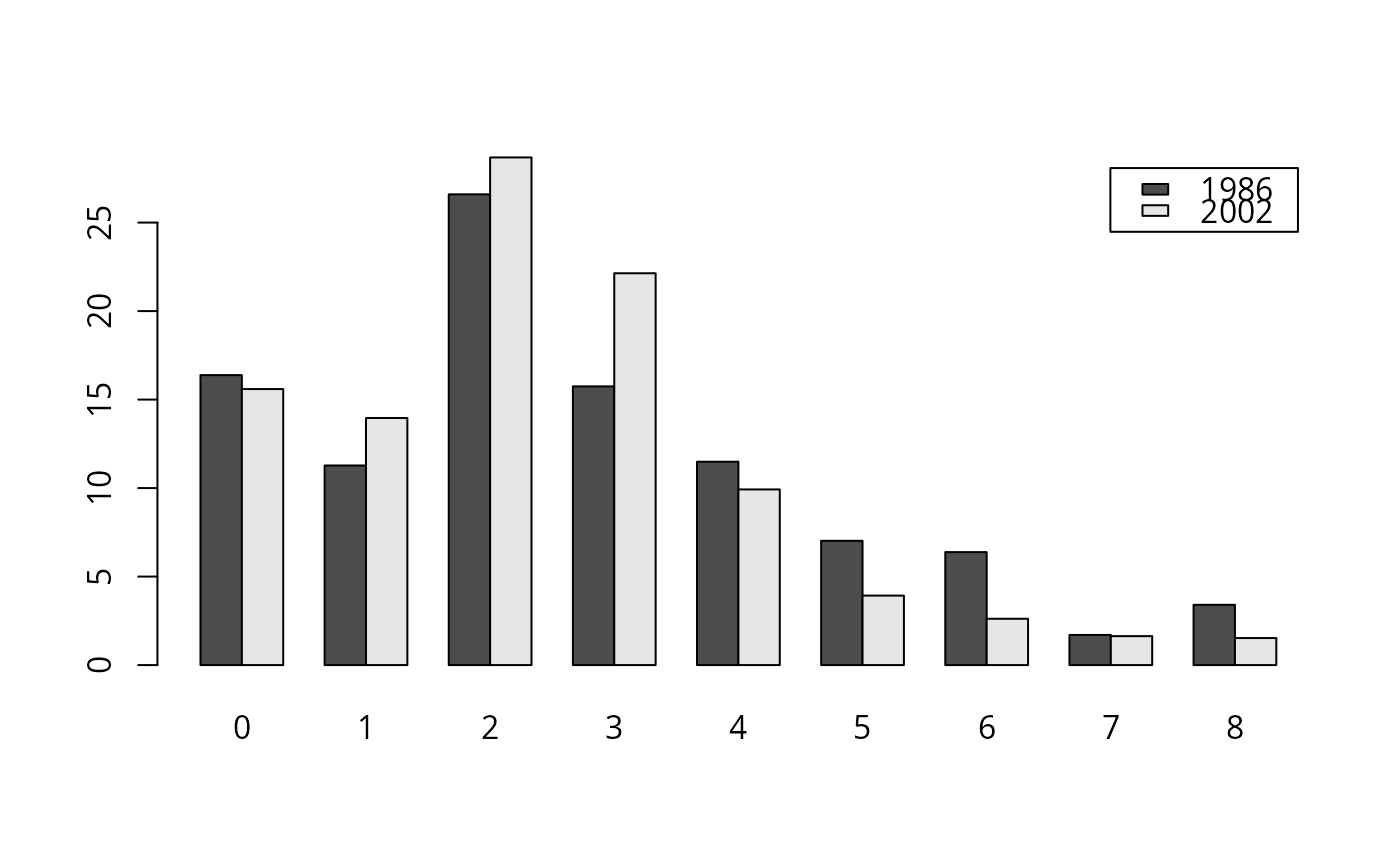
#> kids 1986 2002
#> 0 16.38 15.59
#> 1 11.28 13.96
#> 2 26.60 28.68
#> 3 15.74 22.14
#> 4 11.49 9.92
#> 5 7.02 3.93
#> 6 6.38 2.62
#> 7 1.70 1.64
#> 8 3.40 1.53
## Figure 2.1
barplot(t(kids_tab[, c(4, 8)]), beside = TRUE, legend = TRUE)
 ## Chapter 3, Example 3.14
## Table 3.1
gss40$nokids <- factor(gss40$kids <= 0,
levels = c(FALSE, TRUE), labels = c("no", "yes"))
nokids_p1 <- glm(nokids ~ 1, data = gss40, family = binomial(link = "probit"))
nokids_p2 <- glm(nokids ~ trend, data = gss40, family = binomial(link = "probit"))
nokids_p3 <- glm(nokids ~ trend + education + ethnicity + siblings,
data = gss40, family = binomial(link = "probit"))
## p. 87
lrtest(nokids_p1, nokids_p2, nokids_p3)
#> Likelihood ratio test
#>
#> Model 1: nokids ~ 1
#> Model 2: nokids ~ trend
#> Model 3: nokids ~ trend + education + ethnicity + siblings
#> #Df LogLik Df Chisq Pr(>Chisq)
#> 1 1 -2126.9
#> 2 2 -2123.6 1 6.5677 0.01038 *
#> 3 5 -2107.1 3 32.9906 3.235e-07 ***
#> ---
#> Signif. codes: 0 ‘***’ 0.001 ‘**’ 0.01 ‘*’ 0.05 ‘.’ 0.1 ‘ ’ 1
## Chapter 4, Example 4.1
gss40$nokids01 <- as.numeric(gss40$nokids) - 1
nokids_lm3 <- lm(nokids01 ~ trend + education + ethnicity + siblings, data = gss40)
coeftest(nokids_lm3, vcov = sandwich)
#>
#> t test of coefficients:
#>
#> Estimate Std. Error t value Pr(>|t|)
#> (Intercept) 0.03972864 0.02898580 1.3706 0.1706
#> trend 0.00060242 0.00053829 1.1191 0.2631
#> education 0.00757341 0.00187637 4.0362 5.511e-05 ***
#> ethnicitycauc 0.01424775 0.01314836 1.0836 0.2786
#> siblings -0.00235388 0.00153770 -1.5308 0.1259
#> ---
#> Signif. codes: 0 ‘***’ 0.001 ‘**’ 0.01 ‘*’ 0.05 ‘.’ 0.1 ‘ ’ 1
#>
## Example 4.3
## Table 4.1
nokids_l1 <- glm(nokids ~ 1, data = gss40, family = binomial(link = "logit"))
nokids_l3 <- glm(nokids ~ trend + education + ethnicity + siblings,
data = gss40, family = binomial(link = "logit"))
lrtest(nokids_p3)
#> Error in eval(mf, parent.frame()): object 'gss40' not found
lrtest(nokids_l3)
#> Error in eval(mf, parent.frame()): object 'gss40' not found
## Table 4.2
nokids_xbar <- colMeans(model.matrix(nokids_l3))
sum(coef(nokids_p3) * nokids_xbar)
#> [1] -1.069858
sum(coef(nokids_l3) * nokids_xbar)
#> [1] -1.802965
dnorm(sum(coef(nokids_p3) * nokids_xbar))
#> [1] 0.2250941
dlogis(sum(coef(nokids_l3) * nokids_xbar))
#> [1] 0.1214709
dnorm(sum(coef(nokids_p3) * nokids_xbar)) * coef(nokids_p3)[3]
#> education
#> 0.007072723
dlogis(sum(coef(nokids_l3) * nokids_xbar)) * coef(nokids_l3)[3]
#> education
#> 0.007658209
exp(coef(nokids_l3)[3])
#> education
#> 1.065075
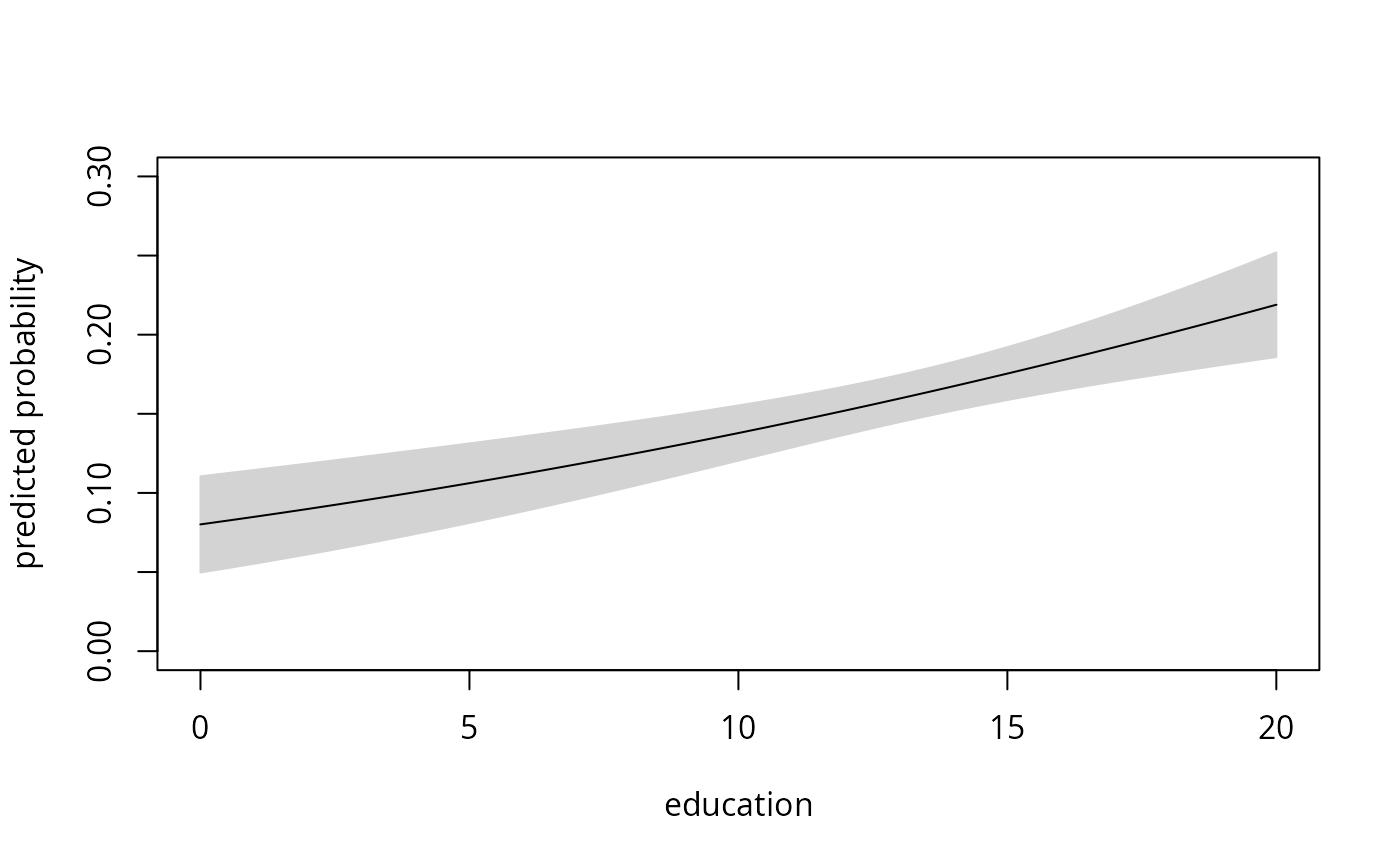
## Figure 4.4
## everything by hand (for ethnicity = "cauc" group)
nokids_xbar <- as.vector(nokids_xbar)
nokids_nd <- data.frame(education = seq(0, 20, by = 0.5), trend = nokids_xbar[2],
ethnicity = "cauc", siblings = nokids_xbar[4])
nokids_p3_fit <- predict(nokids_p3, newdata = nokids_nd,
type = "response", se.fit = TRUE)
plot(nokids_nd$education, nokids_p3_fit$fit, type = "l",
xlab = "education", ylab = "predicted probability", ylim = c(0, 0.3))
polygon(c(nokids_nd$education, rev(nokids_nd$education)),
c(nokids_p3_fit$fit + 1.96 * nokids_p3_fit$se.fit,
rev(nokids_p3_fit$fit - 1.96 * nokids_p3_fit$se.fit)),
col = "lightgray", border = "lightgray")
lines(nokids_nd$education, nokids_p3_fit$fit)
## Chapter 3, Example 3.14
## Table 3.1
gss40$nokids <- factor(gss40$kids <= 0,
levels = c(FALSE, TRUE), labels = c("no", "yes"))
nokids_p1 <- glm(nokids ~ 1, data = gss40, family = binomial(link = "probit"))
nokids_p2 <- glm(nokids ~ trend, data = gss40, family = binomial(link = "probit"))
nokids_p3 <- glm(nokids ~ trend + education + ethnicity + siblings,
data = gss40, family = binomial(link = "probit"))
## p. 87
lrtest(nokids_p1, nokids_p2, nokids_p3)
#> Likelihood ratio test
#>
#> Model 1: nokids ~ 1
#> Model 2: nokids ~ trend
#> Model 3: nokids ~ trend + education + ethnicity + siblings
#> #Df LogLik Df Chisq Pr(>Chisq)
#> 1 1 -2126.9
#> 2 2 -2123.6 1 6.5677 0.01038 *
#> 3 5 -2107.1 3 32.9906 3.235e-07 ***
#> ---
#> Signif. codes: 0 ‘***’ 0.001 ‘**’ 0.01 ‘*’ 0.05 ‘.’ 0.1 ‘ ’ 1
## Chapter 4, Example 4.1
gss40$nokids01 <- as.numeric(gss40$nokids) - 1
nokids_lm3 <- lm(nokids01 ~ trend + education + ethnicity + siblings, data = gss40)
coeftest(nokids_lm3, vcov = sandwich)
#>
#> t test of coefficients:
#>
#> Estimate Std. Error t value Pr(>|t|)
#> (Intercept) 0.03972864 0.02898580 1.3706 0.1706
#> trend 0.00060242 0.00053829 1.1191 0.2631
#> education 0.00757341 0.00187637 4.0362 5.511e-05 ***
#> ethnicitycauc 0.01424775 0.01314836 1.0836 0.2786
#> siblings -0.00235388 0.00153770 -1.5308 0.1259
#> ---
#> Signif. codes: 0 ‘***’ 0.001 ‘**’ 0.01 ‘*’ 0.05 ‘.’ 0.1 ‘ ’ 1
#>
## Example 4.3
## Table 4.1
nokids_l1 <- glm(nokids ~ 1, data = gss40, family = binomial(link = "logit"))
nokids_l3 <- glm(nokids ~ trend + education + ethnicity + siblings,
data = gss40, family = binomial(link = "logit"))
lrtest(nokids_p3)
#> Error in eval(mf, parent.frame()): object 'gss40' not found
lrtest(nokids_l3)
#> Error in eval(mf, parent.frame()): object 'gss40' not found
## Table 4.2
nokids_xbar <- colMeans(model.matrix(nokids_l3))
sum(coef(nokids_p3) * nokids_xbar)
#> [1] -1.069858
sum(coef(nokids_l3) * nokids_xbar)
#> [1] -1.802965
dnorm(sum(coef(nokids_p3) * nokids_xbar))
#> [1] 0.2250941
dlogis(sum(coef(nokids_l3) * nokids_xbar))
#> [1] 0.1214709
dnorm(sum(coef(nokids_p3) * nokids_xbar)) * coef(nokids_p3)[3]
#> education
#> 0.007072723
dlogis(sum(coef(nokids_l3) * nokids_xbar)) * coef(nokids_l3)[3]
#> education
#> 0.007658209
exp(coef(nokids_l3)[3])
#> education
#> 1.065075
## Figure 4.4
## everything by hand (for ethnicity = "cauc" group)
nokids_xbar <- as.vector(nokids_xbar)
nokids_nd <- data.frame(education = seq(0, 20, by = 0.5), trend = nokids_xbar[2],
ethnicity = "cauc", siblings = nokids_xbar[4])
nokids_p3_fit <- predict(nokids_p3, newdata = nokids_nd,
type = "response", se.fit = TRUE)
plot(nokids_nd$education, nokids_p3_fit$fit, type = "l",
xlab = "education", ylab = "predicted probability", ylim = c(0, 0.3))
polygon(c(nokids_nd$education, rev(nokids_nd$education)),
c(nokids_p3_fit$fit + 1.96 * nokids_p3_fit$se.fit,
rev(nokids_p3_fit$fit - 1.96 * nokids_p3_fit$se.fit)),
col = "lightgray", border = "lightgray")
lines(nokids_nd$education, nokids_p3_fit$fit)
 ## using "effects" package (for average "ethnicity" variable)
library("effects")
nokids_p3_ef <- effect("education", nokids_p3, xlevels = list(education = 0:20))
plot(nokids_p3_ef, rescale.axis = FALSE, ylim = c(0, 0.3))
## using "effects" package (for average "ethnicity" variable)
library("effects")
nokids_p3_ef <- effect("education", nokids_p3, xlevels = list(education = 0:20))
plot(nokids_p3_ef, rescale.axis = FALSE, ylim = c(0, 0.3))
 ## using "effects" plus modification by hand
nokids_p3_ef1 <- as.data.frame(nokids_p3_ef)
plot(pnorm(fit) ~ education, data = nokids_p3_ef1, type = "n", ylim = c(0, 0.3))
polygon(c(0:20, 20:0), pnorm(c(nokids_p3_ef1$upper, rev(nokids_p3_ef1$lower))),
col = "lightgray", border = "lightgray")
lines(pnorm(fit) ~ education, data = nokids_p3_ef1)
## using "effects" plus modification by hand
nokids_p3_ef1 <- as.data.frame(nokids_p3_ef)
plot(pnorm(fit) ~ education, data = nokids_p3_ef1, type = "n", ylim = c(0, 0.3))
polygon(c(0:20, 20:0), pnorm(c(nokids_p3_ef1$upper, rev(nokids_p3_ef1$lower))),
col = "lightgray", border = "lightgray")
lines(pnorm(fit) ~ education, data = nokids_p3_ef1)
 ## Table 4.6
## McFadden's R^2
1 - as.numeric( logLik(nokids_p3) / logLik(nokids_p1) )
#> [1] 0.009299554
1 - as.numeric( logLik(nokids_l3) / logLik(nokids_l1) )
#> [1] 0.009840523
## McKelvey and Zavoina R^2
r2mz <- function(obj) {
ystar <- predict(obj)
sse <- sum((ystar - mean(ystar))^2)
s2 <- switch(obj$family$link, "probit" = 1, "logit" = pi^2/3, NA)
n <- length(residuals(obj))
sse / (n * s2 + sse)
}
r2mz(nokids_p3)
#> [1] 0.01784602
r2mz(nokids_l3)
#> [1] 0.02076783
## AUC
library("ROCR")
nokids_p3_pred <- prediction(fitted(nokids_p3), gss40$nokids)
nokids_l3_pred <- prediction(fitted(nokids_l3), gss40$nokids)
plot(performance(nokids_p3_pred, "tpr", "fpr"))
abline(0, 1, lty = 2)
## Table 4.6
## McFadden's R^2
1 - as.numeric( logLik(nokids_p3) / logLik(nokids_p1) )
#> [1] 0.009299554
1 - as.numeric( logLik(nokids_l3) / logLik(nokids_l1) )
#> [1] 0.009840523
## McKelvey and Zavoina R^2
r2mz <- function(obj) {
ystar <- predict(obj)
sse <- sum((ystar - mean(ystar))^2)
s2 <- switch(obj$family$link, "probit" = 1, "logit" = pi^2/3, NA)
n <- length(residuals(obj))
sse / (n * s2 + sse)
}
r2mz(nokids_p3)
#> [1] 0.01784602
r2mz(nokids_l3)
#> [1] 0.02076783
## AUC
library("ROCR")
nokids_p3_pred <- prediction(fitted(nokids_p3), gss40$nokids)
nokids_l3_pred <- prediction(fitted(nokids_l3), gss40$nokids)
plot(performance(nokids_p3_pred, "tpr", "fpr"))
abline(0, 1, lty = 2)
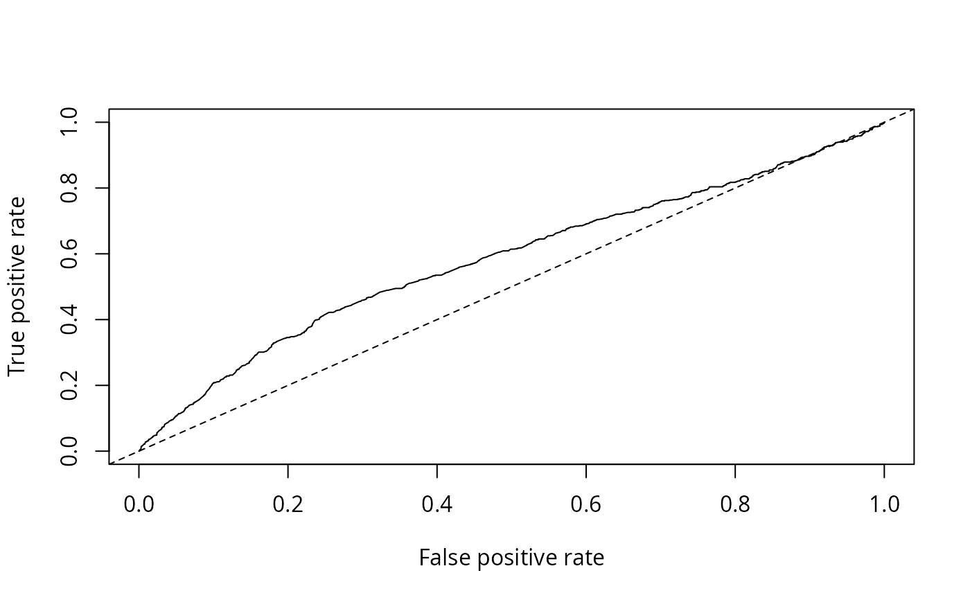 performance(nokids_p3_pred, "auc")
#> A performance instance
#> 'Area under the ROC curve'
plot(performance(nokids_l3_pred, "tpr", "fpr"))
abline(0, 1, lty = 2)
performance(nokids_p3_pred, "auc")
#> A performance instance
#> 'Area under the ROC curve'
plot(performance(nokids_l3_pred, "tpr", "fpr"))
abline(0, 1, lty = 2)
 performance(nokids_l3_pred, "auc")@y.values
#> [[1]]
#> [1] 0.5828855
#>
## Chapter 7
## Table 7.3
## subset selection
gss02 <- subset(GSS7402, year == 2002 & (age < 40 | !is.na(agefirstbirth)))
#Z# This selection conforms with top of page 229. However, there
#Z# are too many observations: 1374. Furthermore, there are six
#Z# observations with agefirstbirth <= 14 which will cause problems in
#Z# taking logs!
## computing time to first birth
gss02$tfb <- with(gss02, ifelse(is.na(agefirstbirth), age - 14, agefirstbirth - 14))
#Z# currently this is still needed before taking logs
gss02$tfb <- pmax(gss02$tfb, 1)
tfb_tobit <- tobit(log(tfb) ~ education + ethnicity + siblings + city16 + immigrant,
data = gss02, left = -Inf, right = log(gss02$age - 14))
tfb_ols <- lm(log(tfb) ~ education + ethnicity + siblings + city16 + immigrant,
data = gss02, subset = !is.na(agefirstbirth))
## Chapter 8
## Example 8.3
gss2002 <- subset(GSS7402, year == 2002 & (agefirstbirth < 40 | age < 40))
gss2002$afb <- with(gss2002, Surv(ifelse(kids > 0, agefirstbirth, age), kids > 0))
afb_km <- survfit(afb ~ 1, data = gss2002)
afb_skm <- summary(afb_km)
print(afb_skm)
#> Call: survfit(formula = afb ~ 1, data = gss2002)
#>
#> time n.risk n.event survival std.err lower 95% CI upper 95% CI
#> 11 1371 1 0.9993 0.000729 0.9978 1.0000
#> 13 1370 3 0.9971 0.001457 0.9942 0.9999
#> 14 1367 2 0.9956 0.001783 0.9921 0.9991
#> 15 1365 14 0.9854 0.003238 0.9791 0.9918
#> 16 1351 40 0.9562 0.005525 0.9455 0.9671
#> 17 1311 66 0.9081 0.007802 0.8929 0.9235
#> 18 1245 97 0.8373 0.009967 0.8180 0.8571
#> 19 1148 106 0.7600 0.011534 0.7378 0.7830
#> 20 1030 122 0.6700 0.012726 0.6455 0.6954
#> 21 898 123 0.5782 0.013406 0.5525 0.6051
#> 22 767 97 0.5051 0.013612 0.4791 0.5325
#> 23 654 72 0.4495 0.013600 0.4236 0.4770
#> 24 563 61 0.4008 0.013480 0.3752 0.4281
#> 25 484 60 0.3511 0.013248 0.3261 0.3781
#> 26 407 45 0.3123 0.012986 0.2878 0.3388
#> 27 351 45 0.2723 0.012618 0.2486 0.2981
#> 28 294 37 0.2380 0.012223 0.2152 0.2632
#> 29 246 32 0.2070 0.011795 0.1852 0.2315
#> 30 209 38 0.1694 0.011119 0.1489 0.1926
#> 31 163 18 0.1507 0.010730 0.1311 0.1733
#> 32 135 19 0.1295 0.010264 0.1108 0.1512
#> 33 108 17 0.1091 0.009766 0.0915 0.1300
#> 34 83 7 0.0999 0.009542 0.0828 0.1205
#> 35 65 13 0.0799 0.009101 0.0639 0.0999
#> 36 45 7 0.0675 0.008815 0.0522 0.0872
#> 37 29 7 0.0512 0.008572 0.0369 0.0711
#> 38 17 3 0.0422 0.008499 0.0284 0.0626
#> 39 12 2 0.0351 0.008411 0.0220 0.0562
with(afb_skm, plot(n.event/n.risk ~ time, type = "s"))
performance(nokids_l3_pred, "auc")@y.values
#> [[1]]
#> [1] 0.5828855
#>
## Chapter 7
## Table 7.3
## subset selection
gss02 <- subset(GSS7402, year == 2002 & (age < 40 | !is.na(agefirstbirth)))
#Z# This selection conforms with top of page 229. However, there
#Z# are too many observations: 1374. Furthermore, there are six
#Z# observations with agefirstbirth <= 14 which will cause problems in
#Z# taking logs!
## computing time to first birth
gss02$tfb <- with(gss02, ifelse(is.na(agefirstbirth), age - 14, agefirstbirth - 14))
#Z# currently this is still needed before taking logs
gss02$tfb <- pmax(gss02$tfb, 1)
tfb_tobit <- tobit(log(tfb) ~ education + ethnicity + siblings + city16 + immigrant,
data = gss02, left = -Inf, right = log(gss02$age - 14))
tfb_ols <- lm(log(tfb) ~ education + ethnicity + siblings + city16 + immigrant,
data = gss02, subset = !is.na(agefirstbirth))
## Chapter 8
## Example 8.3
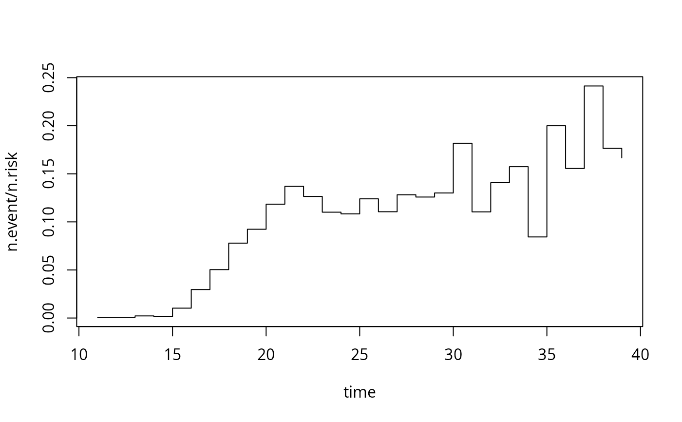
gss2002 <- subset(GSS7402, year == 2002 & (agefirstbirth < 40 | age < 40))
gss2002$afb <- with(gss2002, Surv(ifelse(kids > 0, agefirstbirth, age), kids > 0))
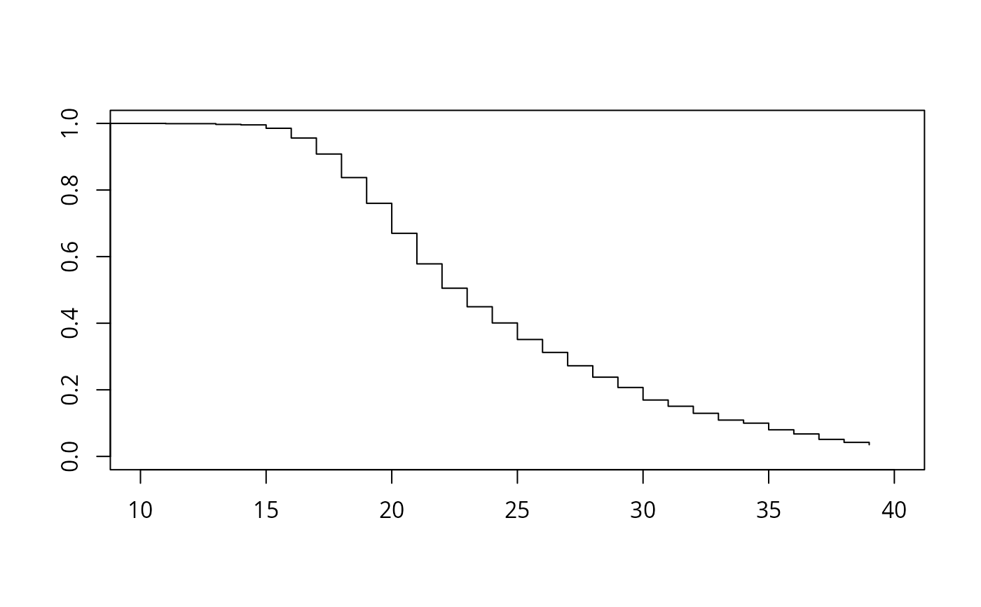
afb_km <- survfit(afb ~ 1, data = gss2002)
afb_skm <- summary(afb_km)
print(afb_skm)
#> Call: survfit(formula = afb ~ 1, data = gss2002)
#>
#> time n.risk n.event survival std.err lower 95% CI upper 95% CI
#> 11 1371 1 0.9993 0.000729 0.9978 1.0000
#> 13 1370 3 0.9971 0.001457 0.9942 0.9999
#> 14 1367 2 0.9956 0.001783 0.9921 0.9991
#> 15 1365 14 0.9854 0.003238 0.9791 0.9918
#> 16 1351 40 0.9562 0.005525 0.9455 0.9671
#> 17 1311 66 0.9081 0.007802 0.8929 0.9235
#> 18 1245 97 0.8373 0.009967 0.8180 0.8571
#> 19 1148 106 0.7600 0.011534 0.7378 0.7830
#> 20 1030 122 0.6700 0.012726 0.6455 0.6954
#> 21 898 123 0.5782 0.013406 0.5525 0.6051
#> 22 767 97 0.5051 0.013612 0.4791 0.5325
#> 23 654 72 0.4495 0.013600 0.4236 0.4770
#> 24 563 61 0.4008 0.013480 0.3752 0.4281
#> 25 484 60 0.3511 0.013248 0.3261 0.3781
#> 26 407 45 0.3123 0.012986 0.2878 0.3388
#> 27 351 45 0.2723 0.012618 0.2486 0.2981
#> 28 294 37 0.2380 0.012223 0.2152 0.2632
#> 29 246 32 0.2070 0.011795 0.1852 0.2315
#> 30 209 38 0.1694 0.011119 0.1489 0.1926
#> 31 163 18 0.1507 0.010730 0.1311 0.1733
#> 32 135 19 0.1295 0.010264 0.1108 0.1512
#> 33 108 17 0.1091 0.009766 0.0915 0.1300
#> 34 83 7 0.0999 0.009542 0.0828 0.1205
#> 35 65 13 0.0799 0.009101 0.0639 0.0999
#> 36 45 7 0.0675 0.008815 0.0522 0.0872
#> 37 29 7 0.0512 0.008572 0.0369 0.0711
#> 38 17 3 0.0422 0.008499 0.0284 0.0626
#> 39 12 2 0.0351 0.008411 0.0220 0.0562
with(afb_skm, plot(n.event/n.risk ~ time, type = "s"))
 plot(afb_km, xlim = c(10, 40), conf.int = FALSE)
 ## Example 8.9
library("survival")
afb_ex <- survreg(
afb ~ education + siblings + ethnicity + immigrant + lowincome16 + city16,
data = gss2002, dist = "exponential")
afb_wb <- survreg(
afb ~ education + siblings + ethnicity + immigrant + lowincome16 + city16,
data = gss2002, dist = "weibull")
afb_ln <- survreg(
afb ~ education + siblings + ethnicity + immigrant + lowincome16 + city16,
data = gss2002, dist = "lognormal")
## Example 8.11
kids_pois <- glm(kids ~ education + trend + ethnicity + immigrant + lowincome16 + city16,
data = gss40, family = poisson)
library("MASS")
kids_nb <- glm.nb(kids ~ education + trend + ethnicity + immigrant + lowincome16 + city16,
data = gss40)
lrtest(kids_pois, kids_nb)
#> Likelihood ratio test
#>
#> Model 1: kids ~ education + trend + ethnicity + immigrant + lowincome16 +
#> city16
#> Model 2: kids ~ education + trend + ethnicity + immigrant + lowincome16 +
#> city16
#> #Df LogLik Df Chisq Pr(>Chisq)
#> 1 7 -10117
#> 2 8 -10014 1 205.17 < 2.2e-16 ***
#> ---
#> Signif. codes: 0 ‘***’ 0.001 ‘**’ 0.01 ‘*’ 0.05 ‘.’ 0.1 ‘ ’ 1
############################################
## German Socio-Economic Panel 1994--2002 ##
############################################
## data
data("GSOEP9402", package = "AER")
## some convenience data transformations
gsoep <- GSOEP9402
gsoep$meducation2 <- cut(gsoep$meducation, breaks = c(6, 10.25, 12.25, 18),
labels = c("7-10", "10.5-12", "12.5-18"))
gsoep$year2 <- factor(gsoep$year)
## Chapter 1
## Table 1.4 plus visualizations
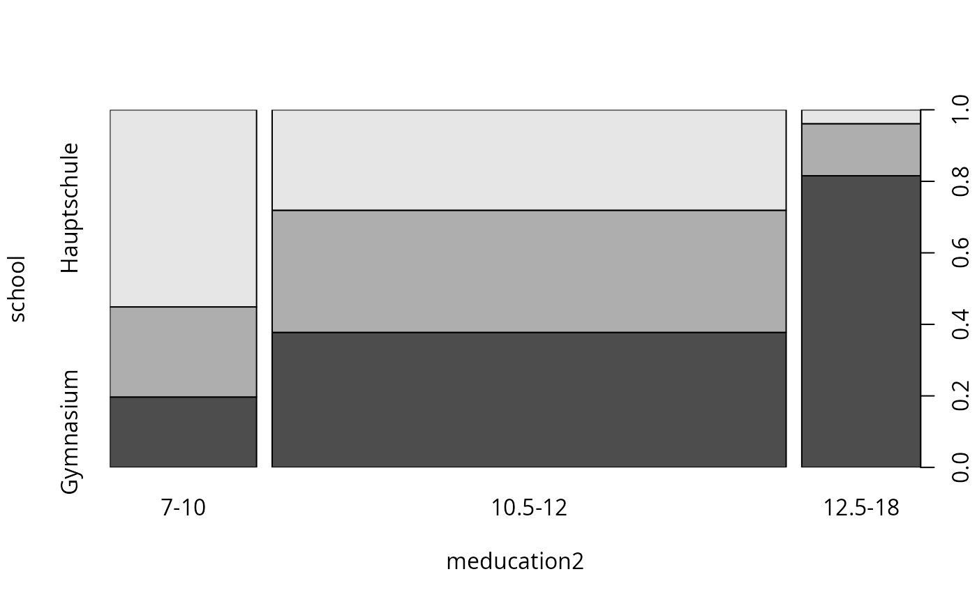
gsoep_tab <- xtabs(~ meducation2 + school, data = gsoep)
round(prop.table(gsoep_tab, 1) * 100, digits = 2)
#> school
#> meducation2 Hauptschule Realschule Gymnasium
#> 7-10 55.12 25.20 19.69
#> 10.5-12 28.09 34.16 37.75
#> 12.5-18 3.88 14.56 81.55
spineplot(gsoep_tab)
## Example 8.9
library("survival")
afb_ex <- survreg(
afb ~ education + siblings + ethnicity + immigrant + lowincome16 + city16,
data = gss2002, dist = "exponential")
afb_wb <- survreg(
afb ~ education + siblings + ethnicity + immigrant + lowincome16 + city16,
data = gss2002, dist = "weibull")
afb_ln <- survreg(
afb ~ education + siblings + ethnicity + immigrant + lowincome16 + city16,
data = gss2002, dist = "lognormal")
## Example 8.11
kids_pois <- glm(kids ~ education + trend + ethnicity + immigrant + lowincome16 + city16,
data = gss40, family = poisson)
library("MASS")
kids_nb <- glm.nb(kids ~ education + trend + ethnicity + immigrant + lowincome16 + city16,
data = gss40)
lrtest(kids_pois, kids_nb)
#> Likelihood ratio test
#>
#> Model 1: kids ~ education + trend + ethnicity + immigrant + lowincome16 +
#> city16
#> Model 2: kids ~ education + trend + ethnicity + immigrant + lowincome16 +
#> city16
#> #Df LogLik Df Chisq Pr(>Chisq)
#> 1 7 -10117
#> 2 8 -10014 1 205.17 < 2.2e-16 ***
#> ---
#> Signif. codes: 0 ‘***’ 0.001 ‘**’ 0.01 ‘*’ 0.05 ‘.’ 0.1 ‘ ’ 1
############################################
## German Socio-Economic Panel 1994--2002 ##
############################################
## data
data("GSOEP9402", package = "AER")
## some convenience data transformations
gsoep <- GSOEP9402
gsoep$meducation2 <- cut(gsoep$meducation, breaks = c(6, 10.25, 12.25, 18),
labels = c("7-10", "10.5-12", "12.5-18"))
gsoep$year2 <- factor(gsoep$year)
## Chapter 1
## Table 1.4 plus visualizations
gsoep_tab <- xtabs(~ meducation2 + school, data = gsoep)
round(prop.table(gsoep_tab, 1) * 100, digits = 2)
#> school
#> meducation2 Hauptschule Realschule Gymnasium
#> 7-10 55.12 25.20 19.69
#> 10.5-12 28.09 34.16 37.75
#> 12.5-18 3.88 14.56 81.55
spineplot(gsoep_tab)
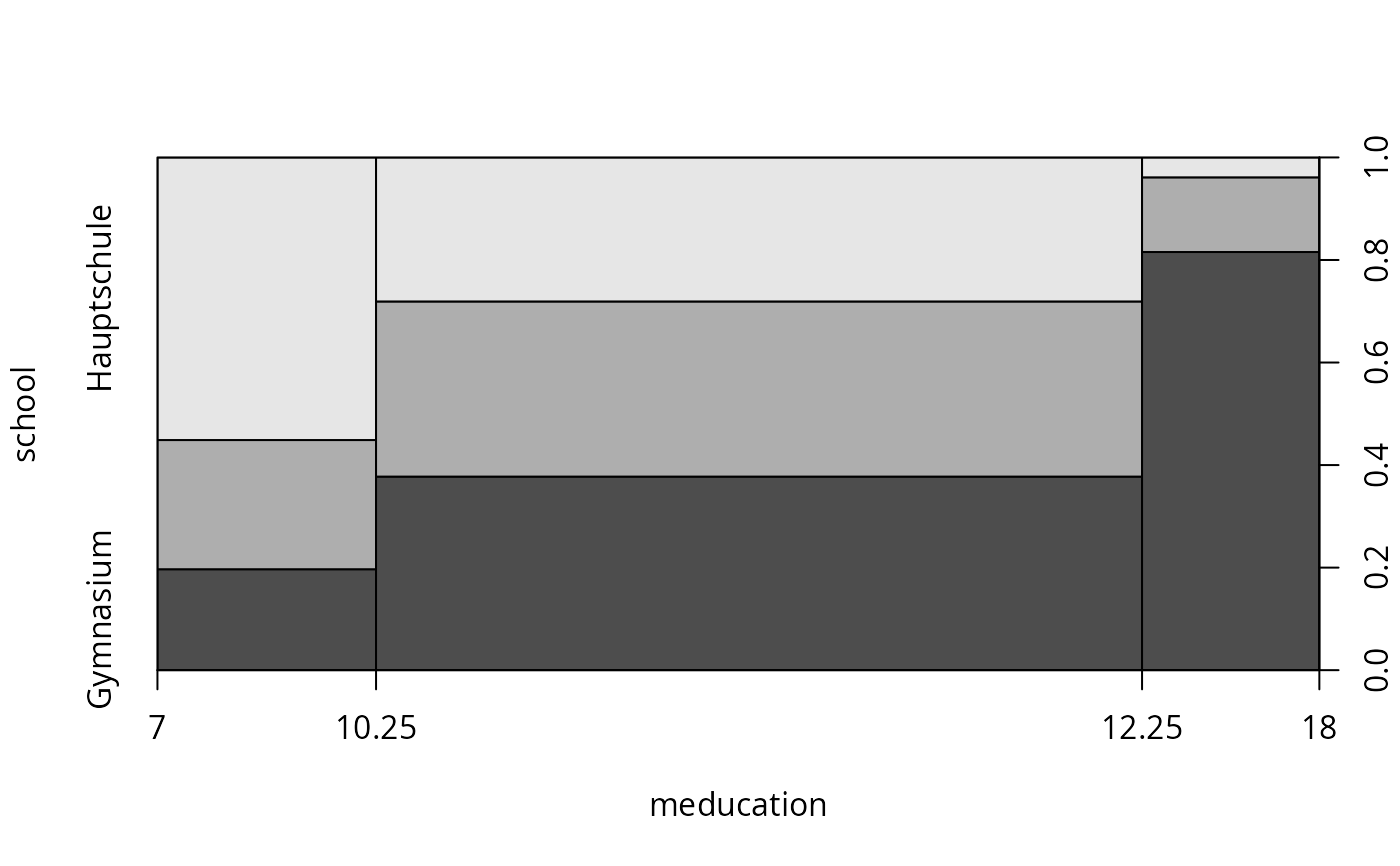
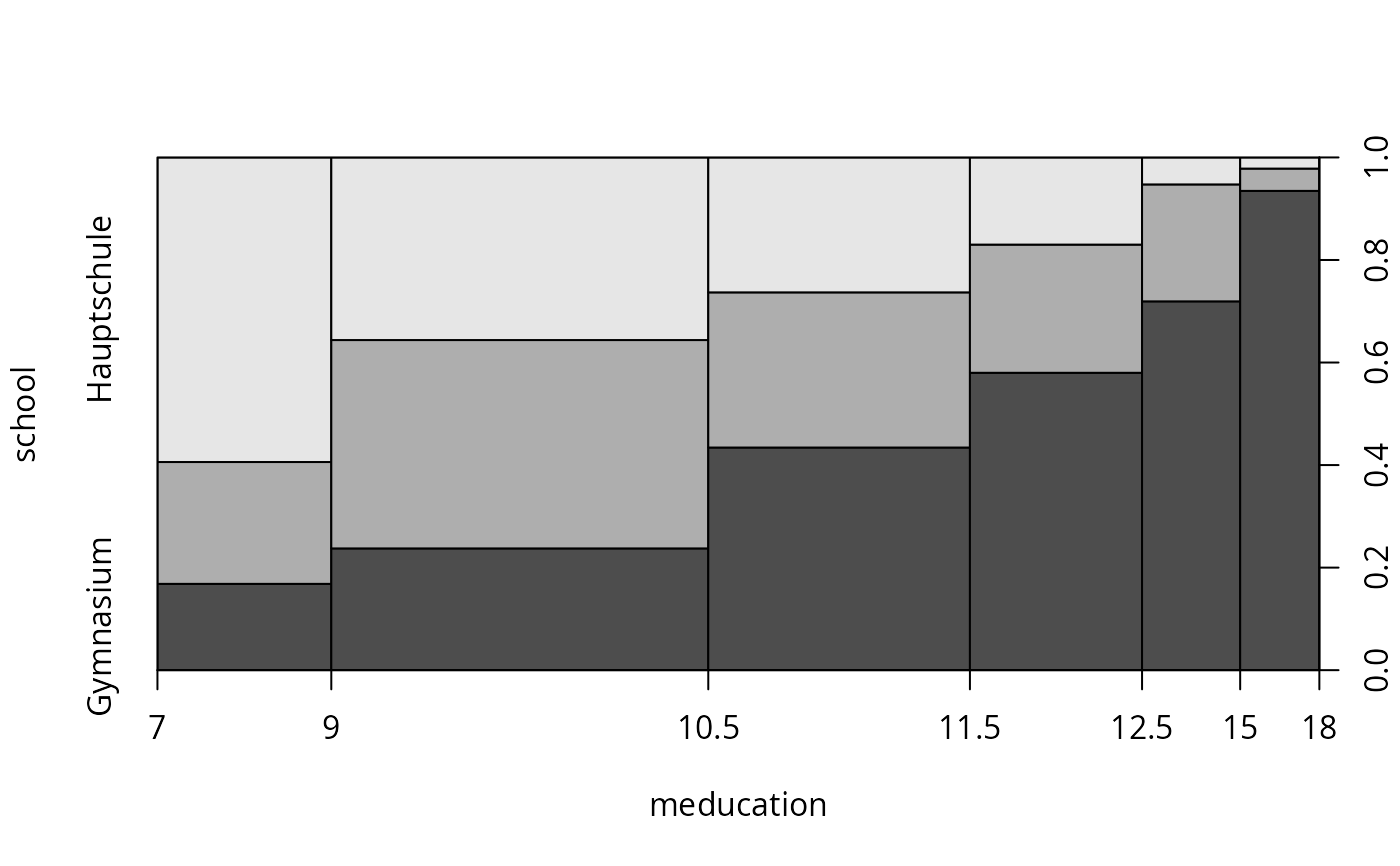
 plot(school ~ meducation, data = gsoep, breaks = c(7, 10.25, 12.25, 18))
 plot(school ~ meducation, data = gsoep, breaks = c(7, 9, 10.5, 11.5, 12.5, 15, 18))
 ## Chapter 5
## Table 5.1
library("nnet")
gsoep_mnl <- multinom(
school ~ meducation + memployment + log(income) + log(size) + parity + year2,
data = gsoep)
#> # weights: 48 (30 variable)
#> initial value 741.563295
#> iter 10 value 655.748279
#> iter 20 value 624.992858
#> iter 30 value 618.605354
#> final value 618.475696
#> converged
coeftest(gsoep_mnl)[c(1:6, 1:6 + 14),]
#> Estimate Std. Error z value Pr(>|z|)
#> Realschule:(Intercept) -6.3864877 2.36903996 -2.6958126 7.021716e-03
#> Realschule:meducation 0.3004843 0.07910641 3.7984819 1.455851e-04
#> Realschule:memploymentparttime 0.4933680 0.32189721 1.5326879 1.253528e-01
#> Realschule:memploymentnone 0.7526399 0.32884476 2.2887392 2.209451e-02
#> Realschule:log(income) 0.3934871 0.22539836 1.7457408 8.085601e-02
#> Realschule:log(size) -1.1921790 0.44641156 -2.6705827 7.571972e-03
#> Realschule:year22002 0.1922413 0.45158350 0.4257049 6.703229e-01
#> Gymnasium:(Intercept) -23.6975758 3.01022807 -7.8723523 3.480345e-15
#> Gymnasium:meducation 0.6597649 0.08144034 8.1012060 5.441700e-16
#> Gymnasium:memploymentparttime 0.9372429 0.34536421 2.7137813 6.652007e-03
#> Gymnasium:memploymentnone 1.1007579 0.35842760 3.0710746 2.132898e-03
#> Gymnasium:log(income) 1.6676745 0.28408439 5.8703492 4.348783e-09
## alternatively
library("mlogit")
gsoep_mnl2 <- mlogit(school ~ 0 | meducation + memployment + log(income) +
log(size) + parity + year2, data = gsoep, shape = "wide", reflevel = "Hauptschule")
coeftest(gsoep_mnl2)[1:12,]
#> Estimate Std. Error t value Pr(>|t|)
#> (Intercept):Gymnasium -23.6982768 3.01026604 -7.872486 1.475202e-14
#> (Intercept):Realschule -6.3865987 2.36904833 -2.695850 7.204061e-03
#> meducation:Gymnasium 0.6597829 0.08144157 8.101304 2.726719e-15
#> meducation:Realschule 0.3004923 0.07910725 3.798543 1.593085e-04
#> memploymentparttime:Gymnasium 0.9372401 0.34536576 2.713761 6.830145e-03
#> memploymentparttime:Realschule 0.4933644 0.32189760 1.532675 1.258463e-01
#> memploymentnone:Gymnasium 1.1007670 0.35842942 3.071084 2.222541e-03
#> memploymentnone:Realschule 0.7526490 0.32884523 2.288764 2.241551e-02
#> log(income):Gymnasium 1.6677258 0.28408738 5.870468 6.954975e-09
#> log(income):Realschule 0.3934899 0.22539876 1.745750 8.133056e-02
#> log(size):Gymnasium -1.5459256 0.48775919 -3.169444 1.599570e-03
#> log(size):Realschule -1.1921835 0.44641174 -2.670592 7.762668e-03
## Table 5.2
library("effects")
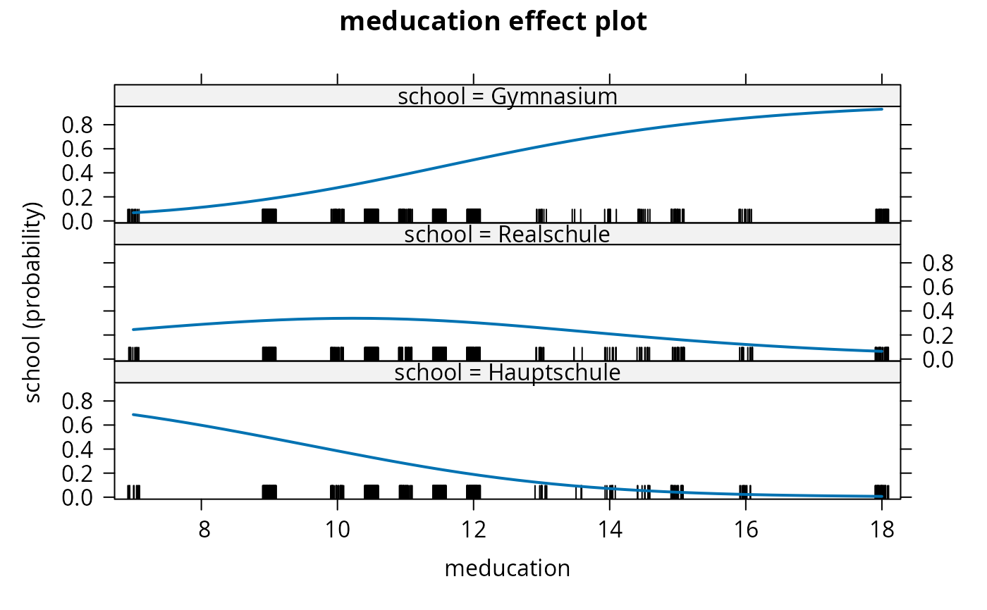
gsoep_eff <- effect("meducation", gsoep_mnl,
xlevels = list(meducation = sort(unique(gsoep$meducation))))
gsoep_eff$prob
#> prob.Hauptschule prob.Realschule prob.Gymnasium
#> [1,] 0.686724467 0.24514452 0.06813102
#> [2,] 0.494486442 0.32195219 0.18356137
#> [3,] 0.385007121 0.33853566 0.27645721
#> [4,] 0.331068546 0.33830072 0.33063074
#> [5,] 0.279605513 0.33203209 0.38836239
#> [6,] 0.231922018 0.32005576 0.44802222
#> [7,] 0.189019319 0.30313717 0.50784351
#> [8,] 0.119575666 0.25898492 0.62143941
#> [9,] 0.093066080 0.23424613 0.67268779
#> [10,] 0.071541719 0.20926168 0.71919660
#> [11,] 0.054404764 0.18493393 0.76066131
#> [12,] 0.040990572 0.16192466 0.79708477
#> [13,] 0.022753542 0.12138826 0.85585820
#> [14,] 0.006601958 0.06423885 0.92915919
plot(gsoep_eff, confint = FALSE)
## Chapter 5
## Table 5.1
library("nnet")
gsoep_mnl <- multinom(
school ~ meducation + memployment + log(income) + log(size) + parity + year2,
data = gsoep)
#> # weights: 48 (30 variable)
#> initial value 741.563295
#> iter 10 value 655.748279
#> iter 20 value 624.992858
#> iter 30 value 618.605354
#> final value 618.475696
#> converged
coeftest(gsoep_mnl)[c(1:6, 1:6 + 14),]
#> Estimate Std. Error z value Pr(>|z|)
#> Realschule:(Intercept) -6.3864877 2.36903996 -2.6958126 7.021716e-03
#> Realschule:meducation 0.3004843 0.07910641 3.7984819 1.455851e-04
#> Realschule:memploymentparttime 0.4933680 0.32189721 1.5326879 1.253528e-01
#> Realschule:memploymentnone 0.7526399 0.32884476 2.2887392 2.209451e-02
#> Realschule:log(income) 0.3934871 0.22539836 1.7457408 8.085601e-02
#> Realschule:log(size) -1.1921790 0.44641156 -2.6705827 7.571972e-03
#> Realschule:year22002 0.1922413 0.45158350 0.4257049 6.703229e-01
#> Gymnasium:(Intercept) -23.6975758 3.01022807 -7.8723523 3.480345e-15
#> Gymnasium:meducation 0.6597649 0.08144034 8.1012060 5.441700e-16
#> Gymnasium:memploymentparttime 0.9372429 0.34536421 2.7137813 6.652007e-03
#> Gymnasium:memploymentnone 1.1007579 0.35842760 3.0710746 2.132898e-03
#> Gymnasium:log(income) 1.6676745 0.28408439 5.8703492 4.348783e-09
## alternatively
library("mlogit")
gsoep_mnl2 <- mlogit(school ~ 0 | meducation + memployment + log(income) +
log(size) + parity + year2, data = gsoep, shape = "wide", reflevel = "Hauptschule")
coeftest(gsoep_mnl2)[1:12,]
#> Estimate Std. Error t value Pr(>|t|)
#> (Intercept):Gymnasium -23.6982768 3.01026604 -7.872486 1.475202e-14
#> (Intercept):Realschule -6.3865987 2.36904833 -2.695850 7.204061e-03
#> meducation:Gymnasium 0.6597829 0.08144157 8.101304 2.726719e-15
#> meducation:Realschule 0.3004923 0.07910725 3.798543 1.593085e-04
#> memploymentparttime:Gymnasium 0.9372401 0.34536576 2.713761 6.830145e-03
#> memploymentparttime:Realschule 0.4933644 0.32189760 1.532675 1.258463e-01
#> memploymentnone:Gymnasium 1.1007670 0.35842942 3.071084 2.222541e-03
#> memploymentnone:Realschule 0.7526490 0.32884523 2.288764 2.241551e-02
#> log(income):Gymnasium 1.6677258 0.28408738 5.870468 6.954975e-09
#> log(income):Realschule 0.3934899 0.22539876 1.745750 8.133056e-02
#> log(size):Gymnasium -1.5459256 0.48775919 -3.169444 1.599570e-03
#> log(size):Realschule -1.1921835 0.44641174 -2.670592 7.762668e-03
## Table 5.2
library("effects")
gsoep_eff <- effect("meducation", gsoep_mnl,
xlevels = list(meducation = sort(unique(gsoep$meducation))))
gsoep_eff$prob
#> prob.Hauptschule prob.Realschule prob.Gymnasium
#> [1,] 0.686724467 0.24514452 0.06813102
#> [2,] 0.494486442 0.32195219 0.18356137
#> [3,] 0.385007121 0.33853566 0.27645721
#> [4,] 0.331068546 0.33830072 0.33063074
#> [5,] 0.279605513 0.33203209 0.38836239
#> [6,] 0.231922018 0.32005576 0.44802222
#> [7,] 0.189019319 0.30313717 0.50784351
#> [8,] 0.119575666 0.25898492 0.62143941
#> [9,] 0.093066080 0.23424613 0.67268779
#> [10,] 0.071541719 0.20926168 0.71919660
#> [11,] 0.054404764 0.18493393 0.76066131
#> [12,] 0.040990572 0.16192466 0.79708477
#> [13,] 0.022753542 0.12138826 0.85585820
#> [14,] 0.006601958 0.06423885 0.92915919
plot(gsoep_eff, confint = FALSE)
 ## Table 5.3, odds
exp(coef(gsoep_mnl)[, "meducation"])
#> Realschule Gymnasium
#> 1.350513 1.934338
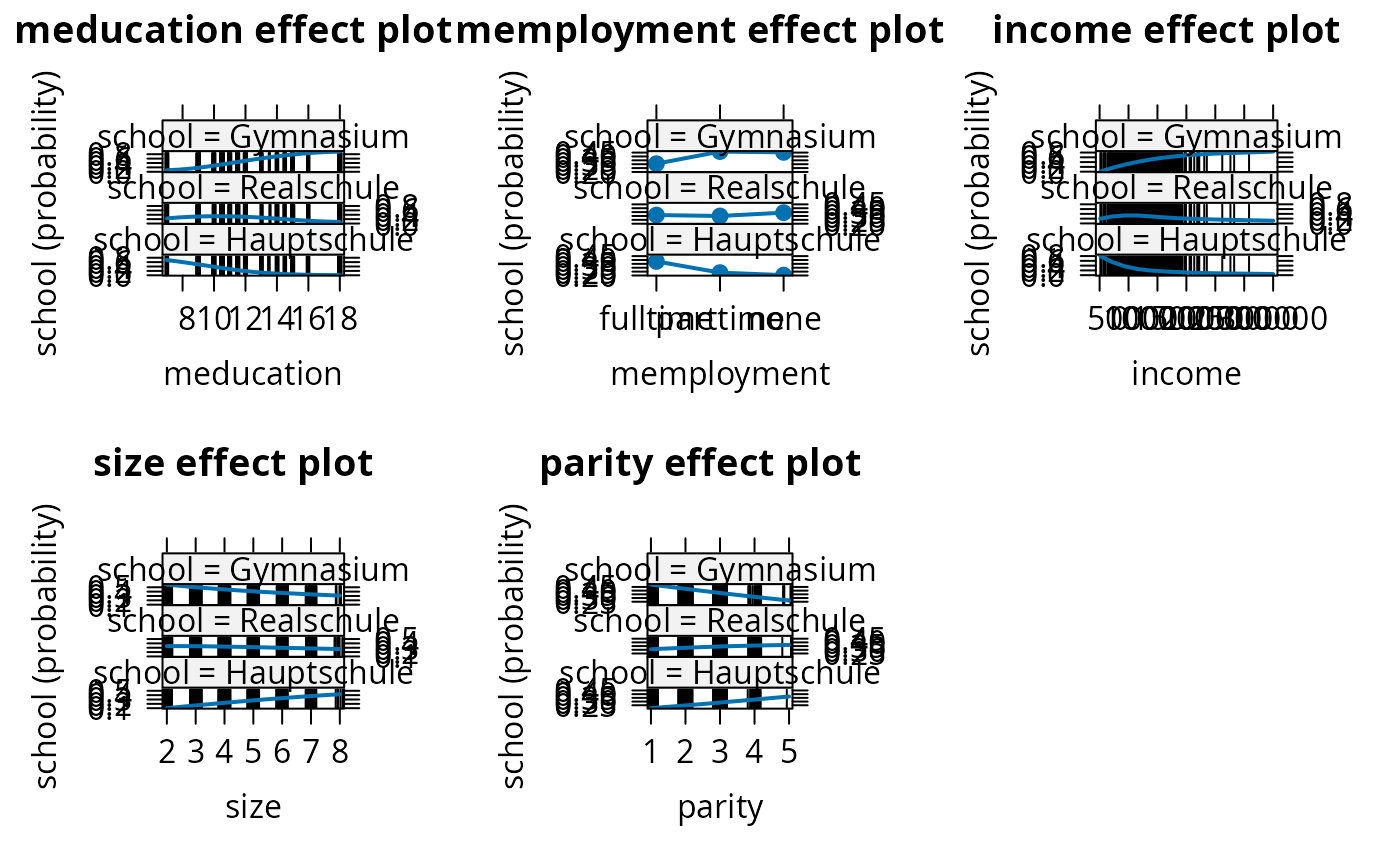
## all effects
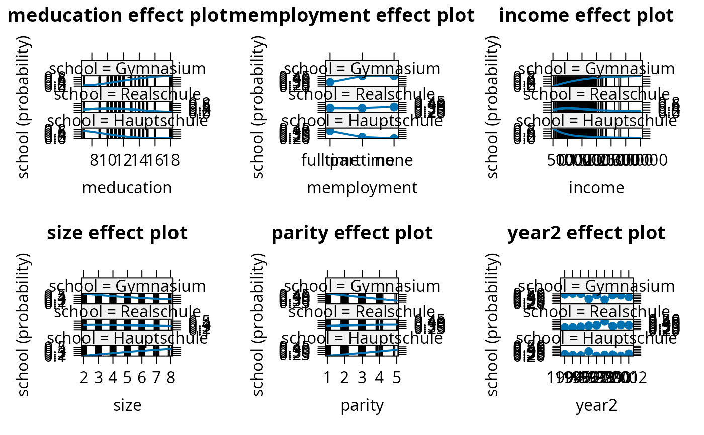
eff_mnl <- allEffects(gsoep_mnl)
plot(eff_mnl, ask = FALSE, confint = FALSE)
## Table 5.3, odds
exp(coef(gsoep_mnl)[, "meducation"])
#> Realschule Gymnasium
#> 1.350513 1.934338
## all effects
eff_mnl <- allEffects(gsoep_mnl)
plot(eff_mnl, ask = FALSE, confint = FALSE)
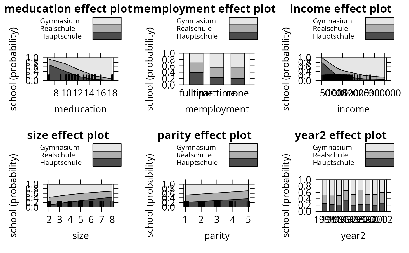
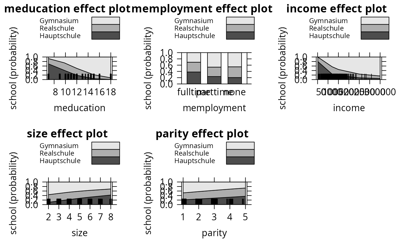
 plot(eff_mnl, ask = FALSE, style = "stacked", colors = gray.colors(3))
 ## omit year
gsoep_mnl1 <- multinom(
school ~ meducation + memployment + log(income) + log(size) + parity,
data = gsoep)
#> # weights: 24 (14 variable)
#> initial value 741.563295
#> iter 10 value 658.442291
#> iter 20 value 624.980518
#> final value 624.957624
#> converged
lrtest(gsoep_mnl, gsoep_mnl1)
#> Likelihood ratio test
#>
#> Model 1: school ~ meducation + memployment + log(income) + log(size) +
#> parity + year2
#> Model 2: school ~ meducation + memployment + log(income) + log(size) +
#> parity
#> #Df LogLik Df Chisq Pr(>Chisq)
#> 1 30 -618.48
#> 2 14 -624.96 -16 12.964 0.6754
eff_mnl1 <- allEffects(gsoep_mnl1)
plot(eff_mnl1, ask = FALSE, confint = FALSE)
## omit year
gsoep_mnl1 <- multinom(
school ~ meducation + memployment + log(income) + log(size) + parity,
data = gsoep)
#> # weights: 24 (14 variable)
#> initial value 741.563295
#> iter 10 value 658.442291
#> iter 20 value 624.980518
#> final value 624.957624
#> converged
lrtest(gsoep_mnl, gsoep_mnl1)
#> Likelihood ratio test
#>
#> Model 1: school ~ meducation + memployment + log(income) + log(size) +
#> parity + year2
#> Model 2: school ~ meducation + memployment + log(income) + log(size) +
#> parity
#> #Df LogLik Df Chisq Pr(>Chisq)
#> 1 30 -618.48
#> 2 14 -624.96 -16 12.964 0.6754
eff_mnl1 <- allEffects(gsoep_mnl1)
plot(eff_mnl1, ask = FALSE, confint = FALSE)
 plot(eff_mnl1, ask = FALSE, style = "stacked", colors = gray.colors(3))
 ## Chapter 6
## Table 6.1
library("MASS")
gsoep$munemp <- factor(gsoep$memployment != "none",
levels = c(FALSE, TRUE), labels = c("no", "yes"))
gsoep_pop <- polr(school ~ meducation + munemp + log(income) + log(size) + parity + year2,
data = gsoep, method = "probit", Hess = TRUE)
gsoep_pol <- polr(school ~ meducation + munemp + log(income) + log(size) + parity + year2,
data = gsoep, Hess = TRUE)
lrtest(gsoep_pop)
#> Error in eval(expr, p): object 'gsoep' not found
lrtest(gsoep_pol)
#> Error in eval(expr, p): object 'gsoep' not found
## Table 6.2
## todo
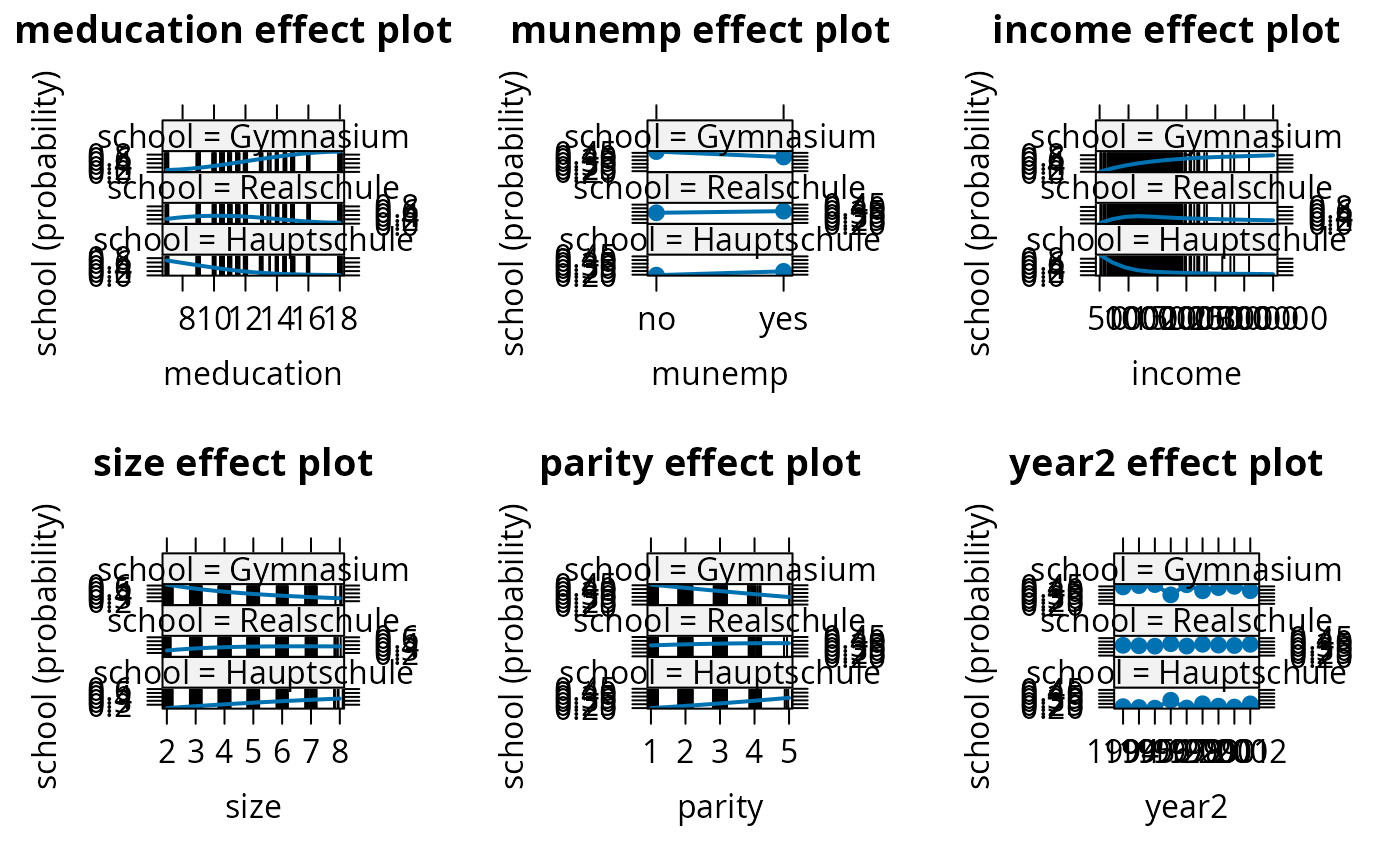
eff_pol <- allEffects(gsoep_pol)
plot(eff_pol, ask = FALSE, confint = FALSE)
## Chapter 6
## Table 6.1
library("MASS")
gsoep$munemp <- factor(gsoep$memployment != "none",
levels = c(FALSE, TRUE), labels = c("no", "yes"))
gsoep_pop <- polr(school ~ meducation + munemp + log(income) + log(size) + parity + year2,
data = gsoep, method = "probit", Hess = TRUE)
gsoep_pol <- polr(school ~ meducation + munemp + log(income) + log(size) + parity + year2,
data = gsoep, Hess = TRUE)
lrtest(gsoep_pop)
#> Error in eval(expr, p): object 'gsoep' not found
lrtest(gsoep_pol)
#> Error in eval(expr, p): object 'gsoep' not found
## Table 6.2
## todo
eff_pol <- allEffects(gsoep_pol)
plot(eff_pol, ask = FALSE, confint = FALSE)
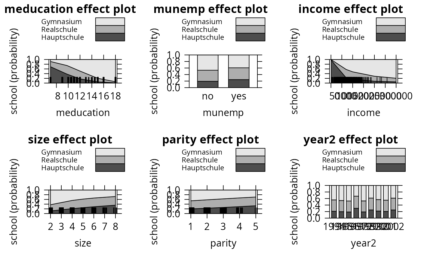
 plot(eff_pol, ask = FALSE, style = "stacked", colors = gray.colors(3))
 ####################################
## Labor Force Participation Data ##
####################################
## Mroz data
data("PSID1976", package = "AER")
PSID1976$nwincome <- with(PSID1976, (fincome - hours * wage)/1000)
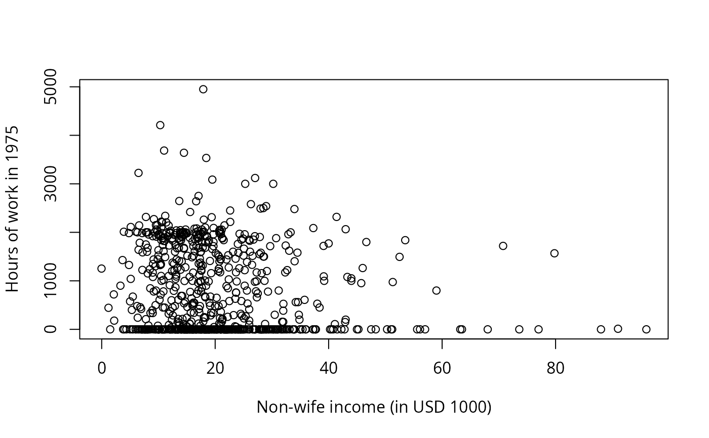
## visualizations
plot(hours ~ nwincome, data = PSID1976,
xlab = "Non-wife income (in USD 1000)",
ylab = "Hours of work in 1975")
####################################
## Labor Force Participation Data ##
####################################
## Mroz data
data("PSID1976", package = "AER")
PSID1976$nwincome <- with(PSID1976, (fincome - hours * wage)/1000)
## visualizations
plot(hours ~ nwincome, data = PSID1976,
xlab = "Non-wife income (in USD 1000)",
ylab = "Hours of work in 1975")
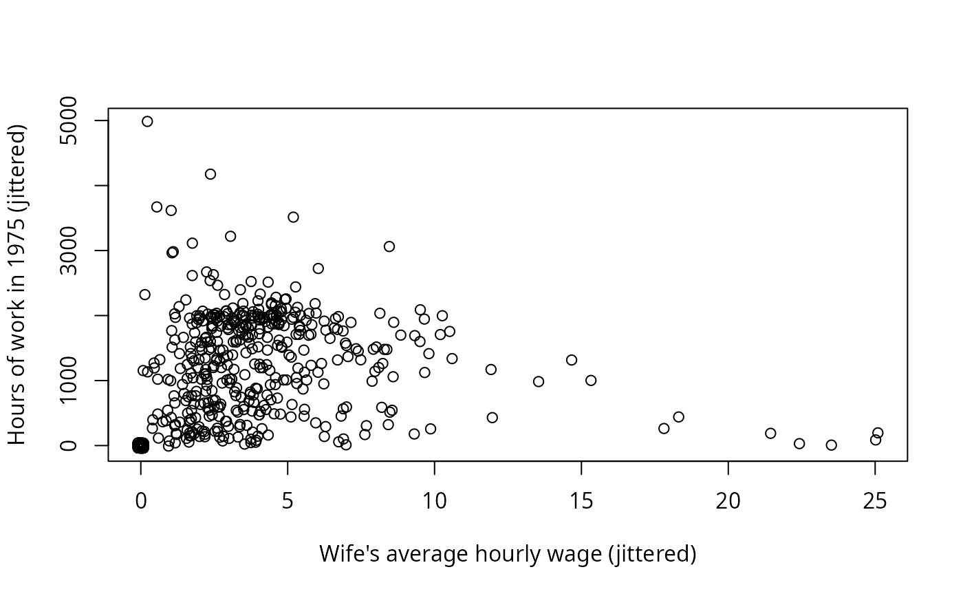
 plot(jitter(hours, 200) ~ jitter(wage, 50), data = PSID1976,
xlab = "Wife's average hourly wage (jittered)",
ylab = "Hours of work in 1975 (jittered)")
plot(jitter(hours, 200) ~ jitter(wage, 50), data = PSID1976,
xlab = "Wife's average hourly wage (jittered)",
ylab = "Hours of work in 1975 (jittered)")
 ## Chapter 1, p. 18
hours_lm <- lm(hours ~ wage + nwincome + youngkids + oldkids, data = PSID1976,
subset = participation == "yes")
## Chapter 7
## Example 7.2, Table 7.1
hours_tobit <- tobit(hours ~ nwincome + education + experience + I(experience^2) +
age + youngkids + oldkids, data = PSID1976)
hours_ols1 <- lm(hours ~ nwincome + education + experience + I(experience^2) +
age + youngkids + oldkids, data = PSID1976)
hours_ols2 <- lm(hours ~ nwincome + education + experience + I(experience^2) +
age + youngkids + oldkids, data = PSID1976, subset = participation == "yes")
## Example 7.10, Table 7.4
wage_ols <- lm(log(wage) ~ education + experience + I(experience^2),
data = PSID1976, subset = participation == "yes")
library("sampleSelection")
wage_ghr <- selection(participation ~ nwincome + age + youngkids + oldkids +
education + experience + I(experience^2),
log(wage) ~ education + experience + I(experience^2), data = PSID1976)
## Exercise 7.13
hours_cragg1 <- glm(participation ~ nwincome + education +
experience + I(experience^2) + age + youngkids + oldkids,
data = PSID1976, family = binomial(link = "probit"))
library("truncreg")
hours_cragg2 <- truncreg(hours ~ nwincome + education +
experience + I(experience^2) + age + youngkids + oldkids,
data = PSID1976, subset = participation == "yes")
## Exercise 7.15
wage_olscoef <- sapply(c(-Inf, 0.5, 1, 1.5, 2), function(censpoint)
coef(lm(log(wage) ~ education + experience + I(experience^2),
data = PSID1976[log(PSID1976$wage) > censpoint,])))
wage_mlcoef <- sapply(c(0.5, 1, 1.5, 2), function(censpoint)
coef(tobit(log(wage) ~ education + experience + I(experience^2),
data = PSID1976, left = censpoint)))
##################################
## Choice of Brand for Crackers ##
##################################
## data
library("mlogit")
data("Cracker", package = "mlogit")
head(Cracker, 3)
#> id disp.sunshine disp.keebler disp.nabisco disp.private feat.sunshine
#> 1 1 0 0 0 0 0
#> 2 1 0 0 0 0 0
#> 3 1 1 0 0 0 0
#> feat.keebler feat.nabisco feat.private price.sunshine price.keebler
#> 1 0 0 0 98 88
#> 2 0 0 0 99 109
#> 3 0 0 0 49 109
#> price.nabisco price.private choice
#> 1 120 71 nabisco
#> 2 99 71 nabisco
#> 3 109 78 sunshine
crack <- mlogit.data(Cracker, varying = 2:13, shape = "wide", choice = "choice")
head(crack, 12)
#> ~~~~~~~
#> first 12 observations out of 13168
#> ~~~~~~~
#> id choice alt disp feat price chid idx
#> 1 1 FALSE keebler 0 0 88 1 1:bler
#> 2 1 TRUE nabisco 0 0 120 1 1:isco
#> 3 1 FALSE private 0 0 71 1 1:vate
#> 4 1 FALSE sunshine 0 0 98 1 1:hine
#> 5 1 FALSE keebler 0 0 109 2 2:bler
#> 6 1 TRUE nabisco 0 0 99 2 2:isco
#> 7 1 FALSE private 0 0 71 2 2:vate
#> 8 1 FALSE sunshine 0 0 99 2 2:hine
#> 9 1 FALSE keebler 0 0 109 3 3:bler
#> 10 1 FALSE nabisco 0 0 109 3 3:isco
#> 11 1 FALSE private 0 0 78 3 3:vate
#> 12 1 TRUE sunshine 1 0 49 3 3:hine
#>
#> ~~~ indexes ~~~~
#> chid alt
#> 1 1 keebler
#> 2 1 nabisco
#> 3 1 private
#> 4 1 sunshine
#> 5 2 keebler
#> 6 2 nabisco
#> 7 2 private
#> 8 2 sunshine
#> 9 3 keebler
#> 10 3 nabisco
#> 11 3 private
#> 12 3 sunshine
#> indexes: 1, 2
## Table 5.6 (model 3 probably not fully converged in W&B)
crack$price <- crack$price/100
crack_mlogit1 <- mlogit(choice ~ price | 0, data = crack, reflevel = "private")
crack_mlogit2 <- mlogit(choice ~ price | 1, data = crack, reflevel = "private")
crack_mlogit3 <- mlogit(choice ~ price + feat + disp | 1, data = crack,
reflevel = "private")
lrtest(crack_mlogit1, crack_mlogit2, crack_mlogit3)
#> Likelihood ratio test
#>
#> Model 1: choice ~ price | 0
#> Model 2: choice ~ price | 1
#> Model 3: choice ~ price + feat + disp | 1
#> #Df LogLik Df Chisq Pr(>Chisq)
#> 1 1 -4498.5
#> 2 4 -3364.9 3 2267.243 < 2.2e-16 ***
#> 3 6 -3347.7 2 34.376 3.43e-08 ***
#> ---
#> Signif. codes: 0 ‘***’ 0.001 ‘**’ 0.01 ‘*’ 0.05 ‘.’ 0.1 ‘ ’ 1
## IIA test
crack_mlogit_all <- update(crack_mlogit2, reflevel = "nabisco")
crack_mlogit_res <- update(crack_mlogit_all,
alt.subset = c("keebler", "nabisco", "sunshine"))
hmftest(crack_mlogit_all, crack_mlogit_res)
#>
#> Hausman-McFadden test
#>
#> data: crack
#> chisq = 51.592, df = 3, p-value = 3.659e-11
#> alternative hypothesis: IIA is rejected
#>
# }
## Chapter 1, p. 18
hours_lm <- lm(hours ~ wage + nwincome + youngkids + oldkids, data = PSID1976,
subset = participation == "yes")
## Chapter 7
## Example 7.2, Table 7.1
hours_tobit <- tobit(hours ~ nwincome + education + experience + I(experience^2) +
age + youngkids + oldkids, data = PSID1976)
hours_ols1 <- lm(hours ~ nwincome + education + experience + I(experience^2) +
age + youngkids + oldkids, data = PSID1976)
hours_ols2 <- lm(hours ~ nwincome + education + experience + I(experience^2) +
age + youngkids + oldkids, data = PSID1976, subset = participation == "yes")
## Example 7.10, Table 7.4
wage_ols <- lm(log(wage) ~ education + experience + I(experience^2),
data = PSID1976, subset = participation == "yes")
library("sampleSelection")
wage_ghr <- selection(participation ~ nwincome + age + youngkids + oldkids +
education + experience + I(experience^2),
log(wage) ~ education + experience + I(experience^2), data = PSID1976)
## Exercise 7.13
hours_cragg1 <- glm(participation ~ nwincome + education +
experience + I(experience^2) + age + youngkids + oldkids,
data = PSID1976, family = binomial(link = "probit"))
library("truncreg")
hours_cragg2 <- truncreg(hours ~ nwincome + education +
experience + I(experience^2) + age + youngkids + oldkids,
data = PSID1976, subset = participation == "yes")
## Exercise 7.15
wage_olscoef <- sapply(c(-Inf, 0.5, 1, 1.5, 2), function(censpoint)
coef(lm(log(wage) ~ education + experience + I(experience^2),
data = PSID1976[log(PSID1976$wage) > censpoint,])))
wage_mlcoef <- sapply(c(0.5, 1, 1.5, 2), function(censpoint)
coef(tobit(log(wage) ~ education + experience + I(experience^2),
data = PSID1976, left = censpoint)))
##################################
## Choice of Brand for Crackers ##
##################################
## data
library("mlogit")
data("Cracker", package = "mlogit")
head(Cracker, 3)
#> id disp.sunshine disp.keebler disp.nabisco disp.private feat.sunshine
#> 1 1 0 0 0 0 0
#> 2 1 0 0 0 0 0
#> 3 1 1 0 0 0 0
#> feat.keebler feat.nabisco feat.private price.sunshine price.keebler
#> 1 0 0 0 98 88
#> 2 0 0 0 99 109
#> 3 0 0 0 49 109
#> price.nabisco price.private choice
#> 1 120 71 nabisco
#> 2 99 71 nabisco
#> 3 109 78 sunshine
crack <- mlogit.data(Cracker, varying = 2:13, shape = "wide", choice = "choice")
head(crack, 12)
#> ~~~~~~~
#> first 12 observations out of 13168
#> ~~~~~~~
#> id choice alt disp feat price chid idx
#> 1 1 FALSE keebler 0 0 88 1 1:bler
#> 2 1 TRUE nabisco 0 0 120 1 1:isco
#> 3 1 FALSE private 0 0 71 1 1:vate
#> 4 1 FALSE sunshine 0 0 98 1 1:hine
#> 5 1 FALSE keebler 0 0 109 2 2:bler
#> 6 1 TRUE nabisco 0 0 99 2 2:isco
#> 7 1 FALSE private 0 0 71 2 2:vate
#> 8 1 FALSE sunshine 0 0 99 2 2:hine
#> 9 1 FALSE keebler 0 0 109 3 3:bler
#> 10 1 FALSE nabisco 0 0 109 3 3:isco
#> 11 1 FALSE private 0 0 78 3 3:vate
#> 12 1 TRUE sunshine 1 0 49 3 3:hine
#>
#> ~~~ indexes ~~~~
#> chid alt
#> 1 1 keebler
#> 2 1 nabisco
#> 3 1 private
#> 4 1 sunshine
#> 5 2 keebler
#> 6 2 nabisco
#> 7 2 private
#> 8 2 sunshine
#> 9 3 keebler
#> 10 3 nabisco
#> 11 3 private
#> 12 3 sunshine
#> indexes: 1, 2
## Table 5.6 (model 3 probably not fully converged in W&B)
crack$price <- crack$price/100
crack_mlogit1 <- mlogit(choice ~ price | 0, data = crack, reflevel = "private")
crack_mlogit2 <- mlogit(choice ~ price | 1, data = crack, reflevel = "private")
crack_mlogit3 <- mlogit(choice ~ price + feat + disp | 1, data = crack,
reflevel = "private")
lrtest(crack_mlogit1, crack_mlogit2, crack_mlogit3)
#> Likelihood ratio test
#>
#> Model 1: choice ~ price | 0
#> Model 2: choice ~ price | 1
#> Model 3: choice ~ price + feat + disp | 1
#> #Df LogLik Df Chisq Pr(>Chisq)
#> 1 1 -4498.5
#> 2 4 -3364.9 3 2267.243 < 2.2e-16 ***
#> 3 6 -3347.7 2 34.376 3.43e-08 ***
#> ---
#> Signif. codes: 0 ‘***’ 0.001 ‘**’ 0.01 ‘*’ 0.05 ‘.’ 0.1 ‘ ’ 1
## IIA test
crack_mlogit_all <- update(crack_mlogit2, reflevel = "nabisco")
crack_mlogit_res <- update(crack_mlogit_all,
alt.subset = c("keebler", "nabisco", "sunshine"))
hmftest(crack_mlogit_all, crack_mlogit_res)
#>
#> Hausman-McFadden test
#>
#> data: crack
#> chisq = 51.592, df = 3, p-value = 3.659e-11
#> alternative hypothesis: IIA is rejected
#>
# }