German Socio-Economic Panel 1994–2002
GSOEP9402.RdCross-section data for 675 14-year old children born between 1980 and 1988. The sample is taken from the German Socio-Economic Panel (GSOEP) for the years 1994 to 2002 to investigate the determinants of secondary school choice.
Usage
data("GSOEP9402")Format
A data frame containing 675 observations on 12 variables.
- school
factor. Child's secondary school level.
- birthyear
Year of child's birth.
- gender
factor indicating child's gender.
- kids
Total number of kids living in household.
- parity
Birth order.
- income
Household income.
- size
Household size
- state
factor indicating German federal state.
- marital
factor indicating mother's marital status.
- meducation
Mother's educational level in years.
- memployment
factor indicating mother's employment level: full-time, part-time, or not working.
- year
Year of GSOEP wave.
Details
This sample from the German Socio-Economic Panel (GSOEP) for the years between 1994 and 2002 has been selected by Winkelmann and Boes (2009) to investigate the determinants of secondary school choice.
In the German schooling system, students are separated relatively early into
different school types, depending on their ability as perceived by the teachers
after four years of primary school. After that, around the age of ten, students are placed
into one of three types of secondary school: "Hauptschule"
(lower secondary school), "Realschule" (middle secondary school), or
"Gymnasium" (upper secondary school). Only a degree from the latter
type of school (called Abitur) provides direct access to universities.
A frequent criticism of this system is that the tracking takes place too early, and that it cements inequalities in education across generations. Although the secondary school choice is based on the teachers' recommendations, it is typically also influenced by the parents; both indirectly through their own educational level and directly through influence on the teachers.
References
Winkelmann, R., and Boes, S. (2009). Analysis of Microdata, 2nd ed. Berlin and Heidelberg: Springer-Verlag.
Examples
#> Loading required namespace: effects
## data
data("GSOEP9402", package = "AER")
## some convenience data transformations
gsoep <- GSOEP9402
gsoep$year2 <- factor(gsoep$year)
## visualization
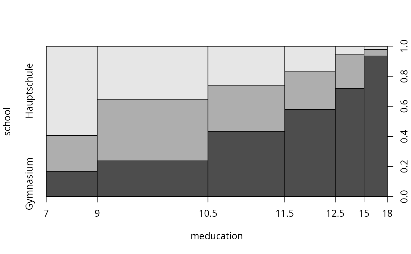
plot(school ~ meducation, data = gsoep, breaks = c(7, 9, 10.5, 11.5, 12.5, 15, 18))
 ## Chapter 5, Table 5.1
library("nnet")
gsoep_mnl <- multinom(
school ~ meducation + memployment + log(income) + log(size) + parity + year2,
data = gsoep)
#> # weights: 48 (30 variable)
#> initial value 741.563295
#> iter 10 value 655.748279
#> iter 20 value 624.992858
#> iter 30 value 618.605354
#> final value 618.475696
#> converged
coeftest(gsoep_mnl)[c(1:6, 1:6 + 14),]
#> Estimate Std. Error z value Pr(>|z|)
#> Realschule:(Intercept) -6.3864877 2.36903996 -2.6958126 7.021716e-03
#> Realschule:meducation 0.3004843 0.07910641 3.7984819 1.455851e-04
#> Realschule:memploymentparttime 0.4933680 0.32189721 1.5326879 1.253528e-01
#> Realschule:memploymentnone 0.7526399 0.32884476 2.2887392 2.209451e-02
#> Realschule:log(income) 0.3934871 0.22539836 1.7457408 8.085601e-02
#> Realschule:log(size) -1.1921790 0.44641156 -2.6705827 7.571972e-03
#> Realschule:year22002 0.1922413 0.45158350 0.4257049 6.703229e-01
#> Gymnasium:(Intercept) -23.6975758 3.01022807 -7.8723523 3.480345e-15
#> Gymnasium:meducation 0.6597649 0.08144034 8.1012060 5.441700e-16
#> Gymnasium:memploymentparttime 0.9372429 0.34536421 2.7137813 6.652007e-03
#> Gymnasium:memploymentnone 1.1007579 0.35842760 3.0710746 2.132898e-03
#> Gymnasium:log(income) 1.6676745 0.28408439 5.8703492 4.348783e-09
## alternatively
library("mlogit")
gsoep_mnl2 <- mlogit(
school ~ 0 | meducation + memployment + log(income) + log(size) + parity + year2,
data = gsoep, shape = "wide", reflevel = "Hauptschule")
coeftest(gsoep_mnl2)[1:12,]
#> Estimate Std. Error t value Pr(>|t|)
#> (Intercept):Gymnasium -23.6982768 3.01026604 -7.872486 1.475202e-14
#> (Intercept):Realschule -6.3865987 2.36904833 -2.695850 7.204061e-03
#> meducation:Gymnasium 0.6597829 0.08144157 8.101304 2.726719e-15
#> meducation:Realschule 0.3004923 0.07910725 3.798543 1.593085e-04
#> memploymentparttime:Gymnasium 0.9372401 0.34536576 2.713761 6.830145e-03
#> memploymentparttime:Realschule 0.4933644 0.32189760 1.532675 1.258463e-01
#> memploymentnone:Gymnasium 1.1007670 0.35842942 3.071084 2.222541e-03
#> memploymentnone:Realschule 0.7526490 0.32884523 2.288764 2.241551e-02
#> log(income):Gymnasium 1.6677258 0.28408738 5.870468 6.954975e-09
#> log(income):Realschule 0.3934899 0.22539876 1.745750 8.133056e-02
#> log(size):Gymnasium -1.5459256 0.48775919 -3.169444 1.599570e-03
#> log(size):Realschule -1.1921835 0.44641174 -2.670592 7.762668e-03
## Table 5.2
library("effects")
#> lattice theme set by effectsTheme()
#> See ?effectsTheme for details.
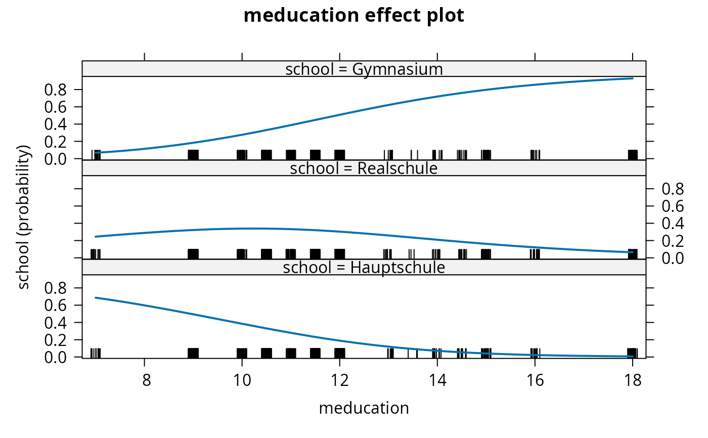
gsoep_eff <- effect("meducation", gsoep_mnl,
xlevels = list(meducation = sort(unique(gsoep$meducation))))
gsoep_eff$prob
#> prob.Hauptschule prob.Realschule prob.Gymnasium
#> [1,] 0.686724467 0.24514452 0.06813102
#> [2,] 0.494486442 0.32195219 0.18356137
#> [3,] 0.385007121 0.33853566 0.27645721
#> [4,] 0.331068546 0.33830072 0.33063074
#> [5,] 0.279605513 0.33203209 0.38836239
#> [6,] 0.231922018 0.32005576 0.44802222
#> [7,] 0.189019319 0.30313717 0.50784351
#> [8,] 0.119575666 0.25898492 0.62143941
#> [9,] 0.093066080 0.23424613 0.67268779
#> [10,] 0.071541719 0.20926168 0.71919660
#> [11,] 0.054404764 0.18493393 0.76066131
#> [12,] 0.040990572 0.16192466 0.79708477
#> [13,] 0.022753542 0.12138826 0.85585820
#> [14,] 0.006601958 0.06423885 0.92915919
plot(gsoep_eff, confint = FALSE)
## Chapter 5, Table 5.1
library("nnet")
gsoep_mnl <- multinom(
school ~ meducation + memployment + log(income) + log(size) + parity + year2,
data = gsoep)
#> # weights: 48 (30 variable)
#> initial value 741.563295
#> iter 10 value 655.748279
#> iter 20 value 624.992858
#> iter 30 value 618.605354
#> final value 618.475696
#> converged
coeftest(gsoep_mnl)[c(1:6, 1:6 + 14),]
#> Estimate Std. Error z value Pr(>|z|)
#> Realschule:(Intercept) -6.3864877 2.36903996 -2.6958126 7.021716e-03
#> Realschule:meducation 0.3004843 0.07910641 3.7984819 1.455851e-04
#> Realschule:memploymentparttime 0.4933680 0.32189721 1.5326879 1.253528e-01
#> Realschule:memploymentnone 0.7526399 0.32884476 2.2887392 2.209451e-02
#> Realschule:log(income) 0.3934871 0.22539836 1.7457408 8.085601e-02
#> Realschule:log(size) -1.1921790 0.44641156 -2.6705827 7.571972e-03
#> Realschule:year22002 0.1922413 0.45158350 0.4257049 6.703229e-01
#> Gymnasium:(Intercept) -23.6975758 3.01022807 -7.8723523 3.480345e-15
#> Gymnasium:meducation 0.6597649 0.08144034 8.1012060 5.441700e-16
#> Gymnasium:memploymentparttime 0.9372429 0.34536421 2.7137813 6.652007e-03
#> Gymnasium:memploymentnone 1.1007579 0.35842760 3.0710746 2.132898e-03
#> Gymnasium:log(income) 1.6676745 0.28408439 5.8703492 4.348783e-09
## alternatively
library("mlogit")
gsoep_mnl2 <- mlogit(
school ~ 0 | meducation + memployment + log(income) + log(size) + parity + year2,
data = gsoep, shape = "wide", reflevel = "Hauptschule")
coeftest(gsoep_mnl2)[1:12,]
#> Estimate Std. Error t value Pr(>|t|)
#> (Intercept):Gymnasium -23.6982768 3.01026604 -7.872486 1.475202e-14
#> (Intercept):Realschule -6.3865987 2.36904833 -2.695850 7.204061e-03
#> meducation:Gymnasium 0.6597829 0.08144157 8.101304 2.726719e-15
#> meducation:Realschule 0.3004923 0.07910725 3.798543 1.593085e-04
#> memploymentparttime:Gymnasium 0.9372401 0.34536576 2.713761 6.830145e-03
#> memploymentparttime:Realschule 0.4933644 0.32189760 1.532675 1.258463e-01
#> memploymentnone:Gymnasium 1.1007670 0.35842942 3.071084 2.222541e-03
#> memploymentnone:Realschule 0.7526490 0.32884523 2.288764 2.241551e-02
#> log(income):Gymnasium 1.6677258 0.28408738 5.870468 6.954975e-09
#> log(income):Realschule 0.3934899 0.22539876 1.745750 8.133056e-02
#> log(size):Gymnasium -1.5459256 0.48775919 -3.169444 1.599570e-03
#> log(size):Realschule -1.1921835 0.44641174 -2.670592 7.762668e-03
## Table 5.2
library("effects")
#> lattice theme set by effectsTheme()
#> See ?effectsTheme for details.
gsoep_eff <- effect("meducation", gsoep_mnl,
xlevels = list(meducation = sort(unique(gsoep$meducation))))
gsoep_eff$prob
#> prob.Hauptschule prob.Realschule prob.Gymnasium
#> [1,] 0.686724467 0.24514452 0.06813102
#> [2,] 0.494486442 0.32195219 0.18356137
#> [3,] 0.385007121 0.33853566 0.27645721
#> [4,] 0.331068546 0.33830072 0.33063074
#> [5,] 0.279605513 0.33203209 0.38836239
#> [6,] 0.231922018 0.32005576 0.44802222
#> [7,] 0.189019319 0.30313717 0.50784351
#> [8,] 0.119575666 0.25898492 0.62143941
#> [9,] 0.093066080 0.23424613 0.67268779
#> [10,] 0.071541719 0.20926168 0.71919660
#> [11,] 0.054404764 0.18493393 0.76066131
#> [12,] 0.040990572 0.16192466 0.79708477
#> [13,] 0.022753542 0.12138826 0.85585820
#> [14,] 0.006601958 0.06423885 0.92915919
plot(gsoep_eff, confint = FALSE)
 ## omit year
gsoep_mnl1 <- multinom(
school ~ meducation + memployment + log(income) + log(size) + parity,
data = gsoep)
#> # weights: 24 (14 variable)
#> initial value 741.563295
#> iter 10 value 658.442291
#> iter 20 value 624.980518
#> final value 624.957624
#> converged
lrtest(gsoep_mnl, gsoep_mnl1)
#> Likelihood ratio test
#>
#> Model 1: school ~ meducation + memployment + log(income) + log(size) +
#> parity + year2
#> Model 2: school ~ meducation + memployment + log(income) + log(size) +
#> parity
#> #Df LogLik Df Chisq Pr(>Chisq)
#> 1 30 -618.48
#> 2 14 -624.96 -16 12.964 0.6754
## Chapter 6
## Table 6.1
library("MASS")
gsoep_pop <- polr(
school ~ meducation + I(memployment != "none") + log(income) + log(size) + parity + year2,
data = gsoep, method = "probit", Hess = TRUE)
gsoep_pol <- polr(
school ~ meducation + I(memployment != "none") + log(income) + log(size) + parity + year2,
data = gsoep, Hess = TRUE)
## compare polr and multinom via AIC
gsoep_pol1 <- polr(
school ~ meducation + memployment + log(income) + log(size) + parity,
data = gsoep, Hess = TRUE)
AIC(gsoep_pol1, gsoep_mnl)
#> df AIC
#> gsoep_pol1 8 1275.075
#> gsoep_mnl 30 1296.951
## effects
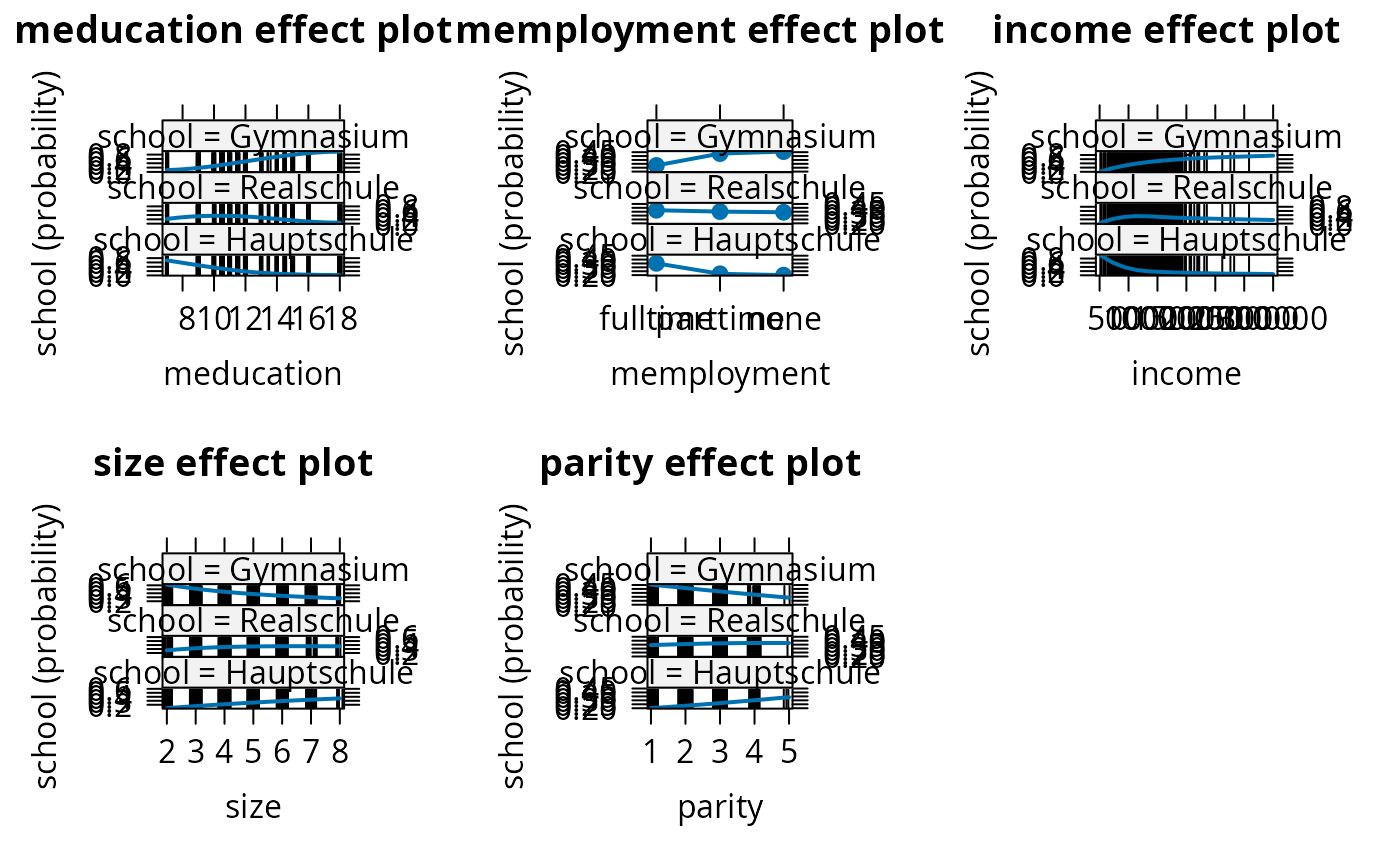
eff_pol1 <- allEffects(gsoep_pol1)
plot(eff_pol1, ask = FALSE, confint = FALSE)
## omit year
gsoep_mnl1 <- multinom(
school ~ meducation + memployment + log(income) + log(size) + parity,
data = gsoep)
#> # weights: 24 (14 variable)
#> initial value 741.563295
#> iter 10 value 658.442291
#> iter 20 value 624.980518
#> final value 624.957624
#> converged
lrtest(gsoep_mnl, gsoep_mnl1)
#> Likelihood ratio test
#>
#> Model 1: school ~ meducation + memployment + log(income) + log(size) +
#> parity + year2
#> Model 2: school ~ meducation + memployment + log(income) + log(size) +
#> parity
#> #Df LogLik Df Chisq Pr(>Chisq)
#> 1 30 -618.48
#> 2 14 -624.96 -16 12.964 0.6754
## Chapter 6
## Table 6.1
library("MASS")
gsoep_pop <- polr(
school ~ meducation + I(memployment != "none") + log(income) + log(size) + parity + year2,
data = gsoep, method = "probit", Hess = TRUE)
gsoep_pol <- polr(
school ~ meducation + I(memployment != "none") + log(income) + log(size) + parity + year2,
data = gsoep, Hess = TRUE)
## compare polr and multinom via AIC
gsoep_pol1 <- polr(
school ~ meducation + memployment + log(income) + log(size) + parity,
data = gsoep, Hess = TRUE)
AIC(gsoep_pol1, gsoep_mnl)
#> df AIC
#> gsoep_pol1 8 1275.075
#> gsoep_mnl 30 1296.951
## effects
eff_pol1 <- allEffects(gsoep_pol1)
plot(eff_pol1, ask = FALSE, confint = FALSE)
 ## More examples can be found in:
## help("WinkelmannBoes2009")
## More examples can be found in:
## help("WinkelmannBoes2009")