Gain capture

gain_capture() is a measure of performance similar to an AUC calculation, but applied to a gain curve.

gain_capture(data, ...)

# S3 method for class 'data.frame'
gain_capture(
  data,
  truth,
  ...,
  estimator = NULL,
  na_rm = TRUE,
  event_level = yardstick_event_level(),
  case_weights = NULL
)

gain_capture_vec(
  truth,
  estimate,
  estimator = NULL,
  na_rm = TRUE,
  event_level = yardstick_event_level(),
  case_weights = NULL,
  ...
)

Arguments

data: A data.frame containing the columns specified by truth and ....
...: A set of unquoted column names or one or more dplyr selector functions to choose which variables contain the class probabilities. If truth is binary, only 1 column should be selected, and it should correspond to the value of event_level. Otherwise, there should be as many columns as factor levels of truth and the ordering of the columns should be the same as the factor levels of truth.
truth: The column identifier for the true class results (that is a factor). This should be an unquoted column name although this argument is passed by expression and supports quasiquotation (you can unquote column names). For _vec() functions, a factor vector.
estimator: One of "binary", "macro", or "macro_weighted" to specify the type of averaging to be done. "binary" is only relevant for the two class case. The other two are general methods for calculating multiclass metrics. The default will automatically choose "binary" or "macro" based on truth.
na_rm: A logical value indicating whether NA values should be stripped before the computation proceeds.
event_level: A single string. Either "first" or "second" to specify which level of truth to consider as the "event". This argument is only applicable when estimator = "binary". The default uses an internal helper that defaults to "first".
case_weights: The optional column identifier for case weights. This should be an unquoted column name that evaluates to a numeric column in data. For _vec() functions, a numeric vector, hardhat::importance_weights(), or hardhat::frequency_weights().
estimate: If truth is binary, a numeric vector of class probabilities corresponding to the "relevant" class. Otherwise, a matrix with as many columns as factor levels of truth. It is assumed that these are in the same order as the levels of truth.

Value

A tibble with columns .metric, .estimator, and .estimate and 1 row of values.

For grouped data frames, the number of rows returned will be the same as the number of groups.

For gain_capture_vec(), a single numeric value (or NA).

Details

gain_capture() calculates the area under the gain curve, but above the baseline, and then divides that by the area under a perfect gain curve, but above the baseline. It is meant to represent the amount of potential gain "captured" by the model.

The gain_capture() metric is identical to the accuracy ratio (AR), which is also sometimes called the gini coefficient. These two are generally calculated on a cumulative accuracy profile curve, but this is the same as a gain curve. See the Engelmann reference for more information.

Relevant Level

There is no common convention on which factor level should automatically be considered the "event" or "positive" result when computing binary classification metrics. In yardstick, the default is to use the first level. To alter this, change the argument event_level to "second" to consider the last level of the factor the level of interest. For multiclass extensions involving one-vs-all comparisons (such as macro averaging), this option is ignored and the "one" level is always the relevant result.

Multiclass

Macro and macro-weighted averaging is available for this metric. The default is to select macro averaging if a truth factor with more than 2 levels is provided. Otherwise, a standard binary calculation is done. See vignette("multiclass", "yardstick") for more information.

References

Engelmann, Bernd & Hayden, Evelyn & Tasche, Dirk (2003). "Measuring the Discriminative Power of Rating Systems," Discussion Paper Series 2: Banking and Financial Studies 2003,01, Deutsche Bundesbank.

Author

Max Kuhn

Examples

# ---------------------------------------------------------------------------
# Two class example

# `truth` is a 2 level factor. The first level is `"Class1"`, which is the
# "event of interest" by default in yardstick. See the Relevant Level
# section above.
data(two_class_example)

# Binary metrics using class probabilities take a factor `truth` column,
# and a single class probability column containing the probabilities of
# the event of interest. Here, since `"Class1"` is the first level of
# `"truth"`, it is the event of interest and we pass in probabilities for it.
gain_capture(two_class_example, truth, Class1)
#> # A tibble: 1 × 3
#>   .metric      .estimator .estimate
#>   <chr>        <chr>          <dbl>
#> 1 gain_capture binary         0.879

# ---------------------------------------------------------------------------
# Multiclass example

# `obs` is a 4 level factor. The first level is `"VF"`, which is the
# "event of interest" by default in yardstick. See the Relevant Level
# section above.
data(hpc_cv)

# You can use the col1:colN tidyselect syntax
library(dplyr)
hpc_cv %>%
  filter(Resample == "Fold01") %>%
  gain_capture(obs, VF:L)
#> # A tibble: 1 × 3
#>   .metric      .estimator .estimate
#>   <chr>        <chr>          <dbl>
#> 1 gain_capture macro          0.743

# Change the first level of `obs` from `"VF"` to `"M"` to alter the
# event of interest. The class probability columns should be supplied
# in the same order as the levels.
hpc_cv %>%
  filter(Resample == "Fold01") %>%
  mutate(obs = relevel(obs, "M")) %>%
  gain_capture(obs, M, VF:L)
#> # A tibble: 1 × 3
#>   .metric      .estimator .estimate
#>   <chr>        <chr>          <dbl>
#> 1 gain_capture macro          0.743

# Groups are respected
hpc_cv %>%
  group_by(Resample) %>%
  gain_capture(obs, VF:L)
#> # A tibble: 10 × 4
#>    Resample .metric      .estimator .estimate
#>    <chr>    <chr>        <chr>          <dbl>
#>  1 Fold01   gain_capture macro          0.743
#>  2 Fold02   gain_capture macro          0.727
#>  3 Fold03   gain_capture macro          0.796
#>  4 Fold04   gain_capture macro          0.748
#>  5 Fold05   gain_capture macro          0.730
#>  6 Fold06   gain_capture macro          0.754
#>  7 Fold07   gain_capture macro          0.730
#>  8 Fold08   gain_capture macro          0.747
#>  9 Fold09   gain_capture macro          0.710
#> 10 Fold10   gain_capture macro          0.731

# Weighted macro averaging
hpc_cv %>%
  group_by(Resample) %>%
  gain_capture(obs, VF:L, estimator = "macro_weighted")
#> # A tibble: 10 × 4
#>    Resample .metric      .estimator     .estimate
#>    <chr>    <chr>        <chr>              <dbl>
#>  1 Fold01   gain_capture macro_weighted     0.759
#>  2 Fold02   gain_capture macro_weighted     0.745
#>  3 Fold03   gain_capture macro_weighted     0.811
#>  4 Fold04   gain_capture macro_weighted     0.734
#>  5 Fold05   gain_capture macro_weighted     0.733
#>  6 Fold06   gain_capture macro_weighted     0.730
#>  7 Fold07   gain_capture macro_weighted     0.737
#>  8 Fold08   gain_capture macro_weighted     0.730
#>  9 Fold09   gain_capture macro_weighted     0.681
#> 10 Fold10   gain_capture macro_weighted     0.737

# Vector version
# Supply a matrix of class probabilities
fold1 <- hpc_cv %>%
  filter(Resample == "Fold01")

gain_capture_vec(
   truth = fold1$obs,
   matrix(
     c(fold1$VF, fold1$F, fold1$M, fold1$L),
     ncol = 4
   )
)
#> [1] 0.7428922

# ---------------------------------------------------------------------------
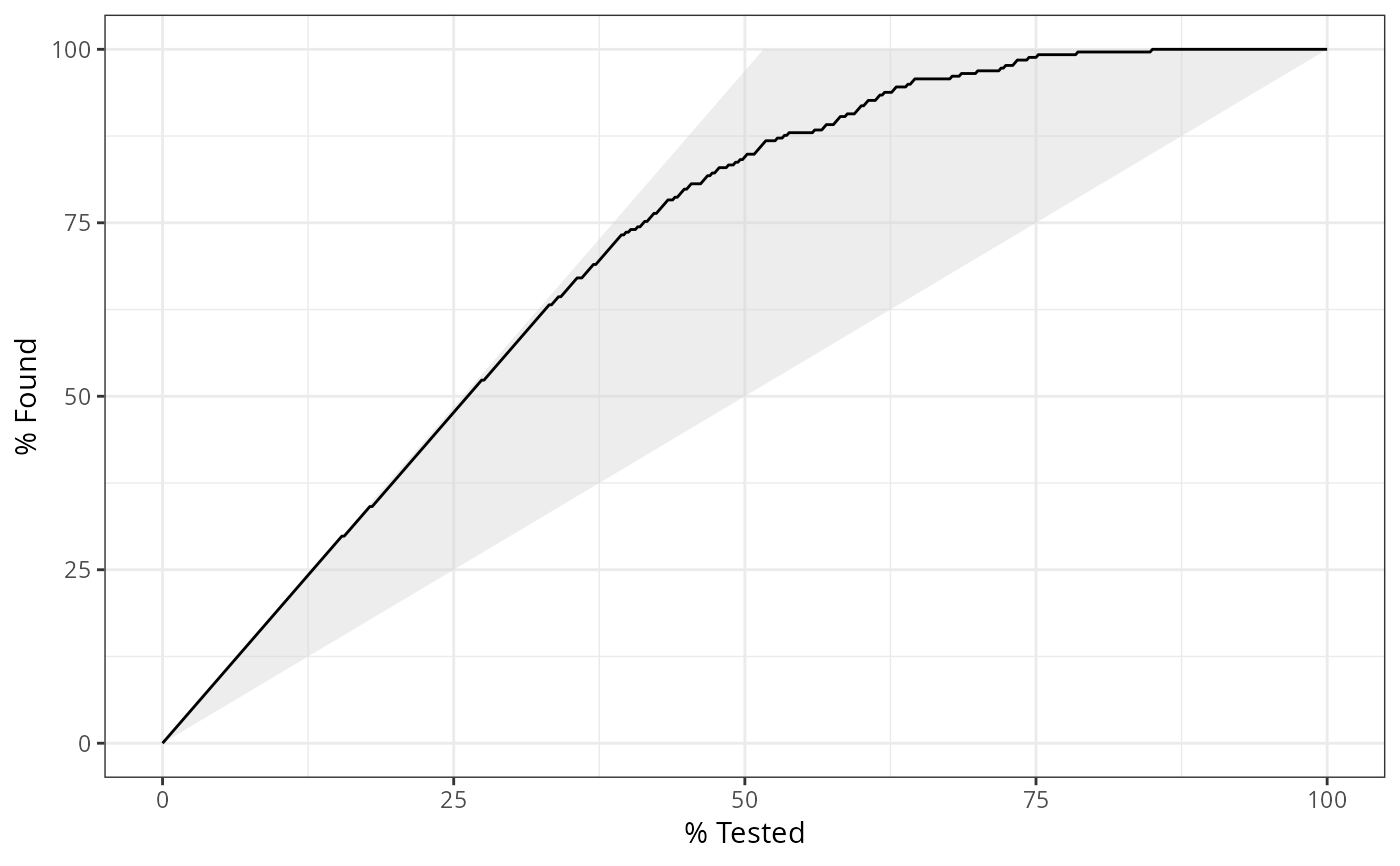
# Visualize gain_capture()

# Visually, this represents the area under the black curve, but above the
# 45 degree line, divided by the area of the shaded triangle.
library(ggplot2)
autoplot(gain_curve(two_class_example, truth, Class1))