Spine Plots and Spinograms
spine.RdSpine plots are a special cases of mosaic plots, and can be seen as a generalization of stacked (or highlighted) bar plots. Analogously, spinograms are an extension of histograms.
spine(x, ...)
# Default S3 method
spine(x, y = NULL,
  breaks = NULL, ylab_tol = 0.05, off = NULL,
  main = "", xlab = NULL, ylab = NULL, ylim = c(0, 1), margins = c(5.1, 4.1, 4.1, 3.1),
  gp = gpar(), name = "spineplot", newpage = TRUE, pop = TRUE,
  ...)
# S3 method for class 'formula'
spine(formula, data = list(),
  breaks = NULL, ylab_tol = 0.05, off = NULL,
  main = "", xlab = NULL, ylab = NULL, ylim = c(0, 1), margins = c(5.1, 4.1, 4.1, 3.1),
  gp = gpar(), name = "spineplot", newpage = TRUE, pop = TRUE,
  ...)
Arguments
- x
an object, the default method expects either a single variable (interpreted to be the explanatory variable) or a 2-way table. See details.
- y
a
"factor"interpreted to be the dependent variable- formula
a
"formula"of typey ~ xwith a single dependent"factor"and a single explanatory variable.- data
an optional data frame.
- breaks
if the explanatory variable is numeric, this controls how it is discretized.
breaksis passed tohistand can be a list of arguments.- ylab_tol
convenience tolerance parameter for y-axis annotation. If the distance between two labels drops under this threshold, they are plotted equidistantly.
- off
vertical offset between the bars (in per cent). It is fixed to
0for spinograms and defaults to2for spine plots.- main, xlab, ylab
character strings for annotation
- ylim
limits for the y axis
- margins
margins when calling
plotViewport- gp
a
"gpar"object controlling the grid graphical parameters of the rectangles. It should specify in particular a vector offillcolors of the same length aslevels(y). The default is to callgray.colors.- name
name of the plotting viewport.
- newpage
logical. Should
grid.newpagebe called before plotting?- pop
logical. Should the viewport created be popped?
- ...
additional arguments passed to
plotViewport.
Details
spine creates either a spinogram or a spine plot. It can be called
via spine(x, y) or spine(y ~ x) where y is interpreted
to be the dependent variable (and has to be categorical) and x
the explanatory variable. x can be either categorical (then a spine
plot is created) or numerical (then a spinogram is plotted).
Additionally, spine can also be called with only a single argument
which then has to be a 2-way table, interpreted to correspond to table(x, y).
Spine plots are a generalization of stacked bar plots where not the heights
but the widths of the bars corresponds to the relative frequencies of x.
The heights of the bars then correspond to the conditional relative frequencies
of y in every x group. This is a special case of a mosaic plot
with specific spacing and shading.
Analogously, spinograms extend stacked histograms. As for the histogram,
x is first discretized (using hist) and then for the
discretized data a spine plot is created.
Value
The table visualized is returned invisibly.
References
Hummel, J. (1996), Linked bar charts: Analysing categorical data graphically. Computational Statistics, 11, 23–33.
Hofmann, H., Theus, M. (2005), Interactive graphics for visualizing conditional distributions, Unpublished Manuscript.
Examples
## Arthritis data (dependence on a categorical variable)
data("Arthritis")
(spine(Improved ~ Treatment, data = Arthritis))
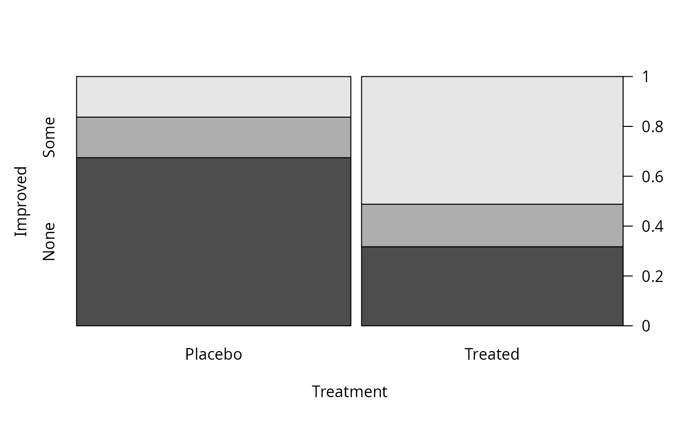 #> Improved
#> Treatment None Some Marked
#> Placebo 29 7 7
#> Treated 13 7 21
## Arthritis data (dependence on a numerical variable)
(spine(Improved ~ Age, data = Arthritis, breaks = 5))
#> Improved
#> Treatment None Some Marked
#> Placebo 29 7 7
#> Treated 13 7 21
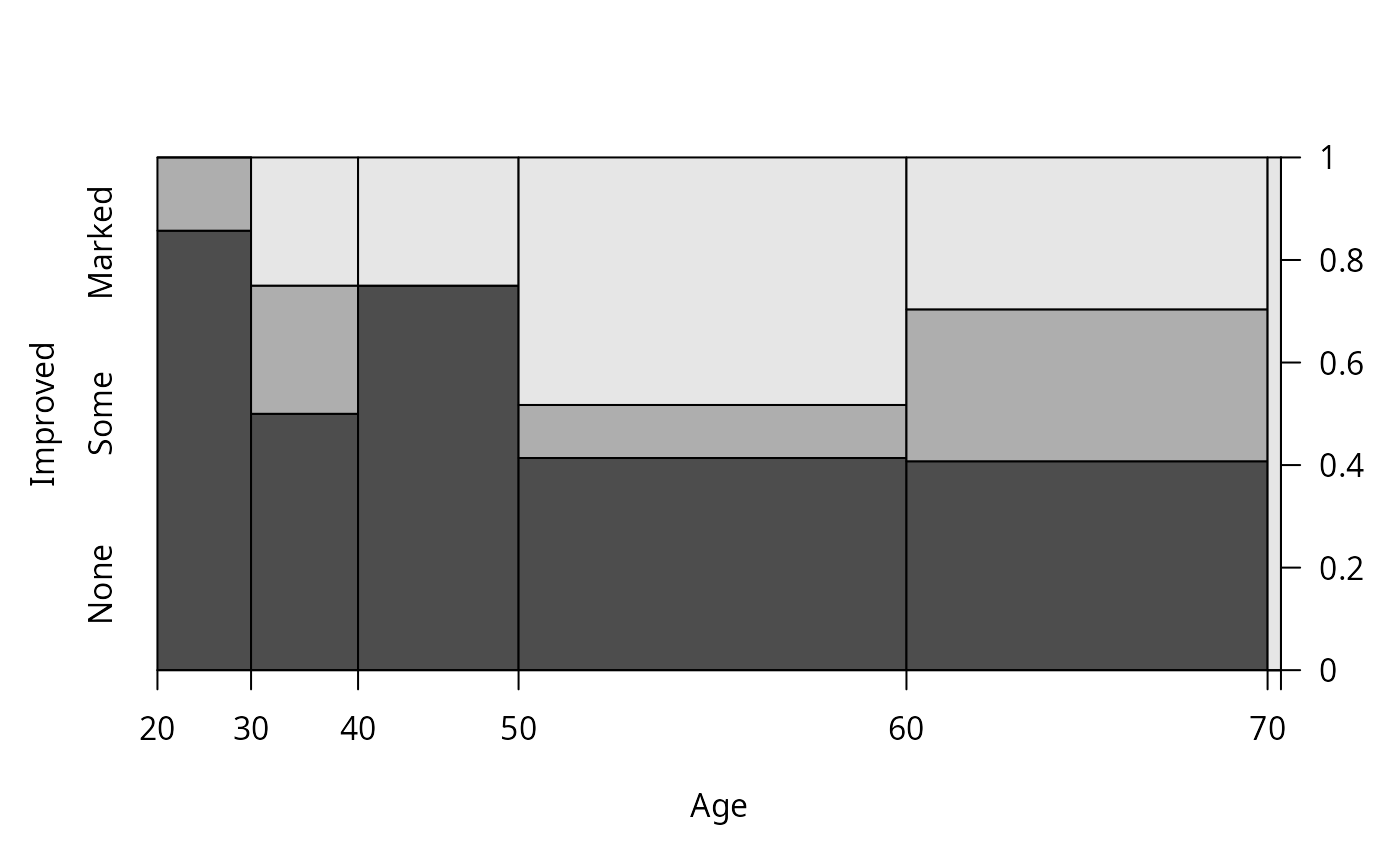
## Arthritis data (dependence on a numerical variable)
(spine(Improved ~ Age, data = Arthritis, breaks = 5))
 #> Improved
#> Age None Some Marked
#> [20,30] 6 1 0
#> (30,40] 4 2 2
#> (40,50] 9 0 3
#> (50,60] 12 3 14
#> (60,70] 11 8 8
#> (70,80] 0 0 1
(spine(Improved ~ Age, data = Arthritis, breaks = quantile(Arthritis$Age)))
#> Improved
#> Age None Some Marked
#> [20,30] 6 1 0
#> (30,40] 4 2 2
#> (40,50] 9 0 3
#> (50,60] 12 3 14
#> (60,70] 11 8 8
#> (70,80] 0 0 1
(spine(Improved ~ Age, data = Arthritis, breaks = quantile(Arthritis$Age)))
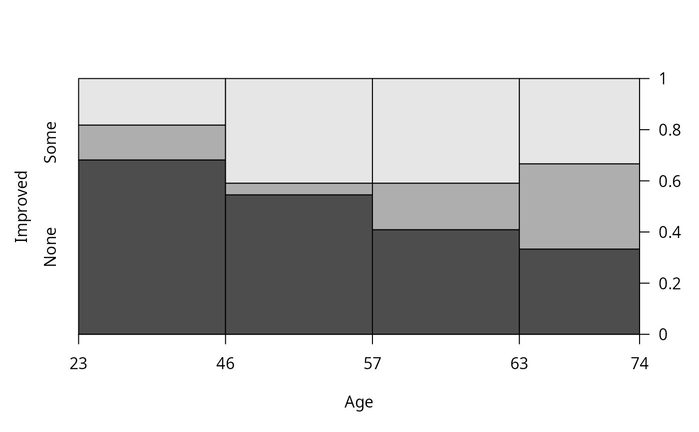 #> Improved
#> Age None Some Marked
#> [23,46] 15 3 4
#> (46,57] 12 1 9
#> (57,63] 9 4 9
#> (63,74] 6 6 6
(spine(Improved ~ Age, data = Arthritis, breaks = "Scott"))
#> Improved
#> Age None Some Marked
#> [23,46] 15 3 4
#> (46,57] 12 1 9
#> (57,63] 9 4 9
#> (63,74] 6 6 6
(spine(Improved ~ Age, data = Arthritis, breaks = "Scott"))
 #> Improved
#> Age None Some Marked
#> [20,30] 6 1 0
#> (30,40] 4 2 2
#> (40,50] 9 0 3
#> (50,60] 12 3 14
#> (60,70] 11 8 8
#> (70,80] 0 0 1
## Space shuttle data (dependence on a numerical variable)
data("SpaceShuttle")
(spine(Fail ~ Temperature, data = SpaceShuttle, breaks = 3))
#> Improved
#> Age None Some Marked
#> [20,30] 6 1 0
#> (30,40] 4 2 2
#> (40,50] 9 0 3
#> (50,60] 12 3 14
#> (60,70] 11 8 8
#> (70,80] 0 0 1
## Space shuttle data (dependence on a numerical variable)
data("SpaceShuttle")
(spine(Fail ~ Temperature, data = SpaceShuttle, breaks = 3))
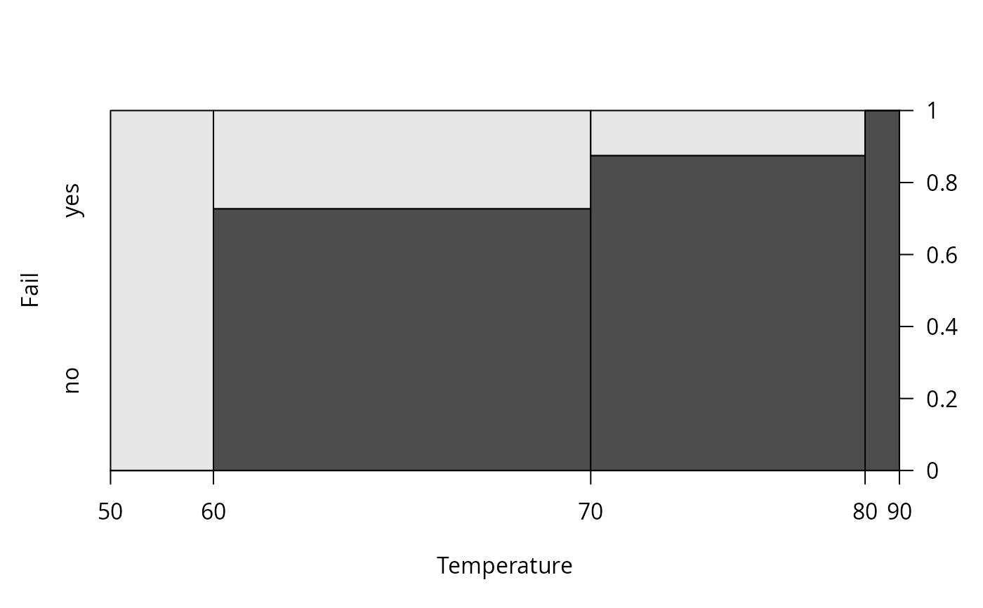 #> Fail
#> Temperature no yes
#> [50,60] 0 3
#> (60,70] 8 3
#> (70,80] 7 1
#> (80,90] 1 0
#> Fail
#> Temperature no yes
#> [50,60] 0 3
#> (60,70] 8 3
#> (70,80] 7 1
#> (80,90] 1 0