Plotting (Log) Odds Ratios

Produces a (conditional) line plot of extended (log) odds ratios.

# S3 method for class 'loddsratio'
plot(x, baseline = TRUE, gp_baseline = gpar(lty = 2),
     lines = TRUE, lwd_lines = 3,
     confidence = TRUE, conf_level = 0.95, lwd_confidence = 2,
     whiskers = 0, transpose = FALSE,
     col = NULL, cex = 0.8, pch = NULL,
     bars = NULL, gp_bars = gpar(fill = "lightgray", alpha = 0.5),
     bar_width = unit(0.05, "npc"),
             
     legend = TRUE, legend_pos = "topright", legend_inset = c(0, 0),
     legend_vgap = unit(0.5, "lines"),
     gp_legend_frame = gpar(lwd = 1, col = "black"),
     gp_legend_title = gpar(fontface = "bold"),
     gp_legend = gpar(), legend_lwd = 1, legend_size = 1,
             
     xlab = NULL, ylab = NULL, xlim = NULL, ylim = NULL,
     main = NULL, gp_main = gpar(fontsize = 12, fontface = "bold"),
     newpage = TRUE, pop = FALSE, return_grob = FALSE,
     add = FALSE, prefix = "", ...)
# S3 method for class 'loddsratio'
lines(x, legend = FALSE, confidence = FALSE, cex = 0, ...)

Arguments

x: an object of class loddsratio.
baseline: if TRUE, a dashed line is plotted at a value of 1 (in case of odds) or 0 (in case of log-odds).
gp_baseline: object of class "gpar" used for the baseline.
lines: if TRUE, the points are connected by lines (only sensible if the variable represented by the x-axis is ordinal).
lwd_lines: Width of the connecting lines (in char units).
confidence: logical; shall confindence intervals be plotted?
conf_level: confidence level used for confidence intervals.
lwd_confidence: Line width of the confidence interval bars (in char units).
whiskers: width of the confidence interval whiskers.
transpose: if TRUE, the plot is transposed.
col: character vector specifying the colors of the fitted lines, by default chosen with rainbow_hcl.
cex: size of the plot symbols (in lines).
pch: character or numeric vector of symbols used for plotting the (possibly conditioned) observed values, recycled as needed.
bars: logical; shall bars be plotted additionally to the points? Defaults to TRUE in case of only one conditioning variable.
gp_bars: object of class "gpar" used for the bars.
bar_width: Width of the bars, if drawn.
legend: logical; if TRUE (default), a legend is drawn.
legend_pos: numeric vector of length 2, specifying x and y coordinates of the legend, or a character string (e.g., "topleft", "center" etc.). Defaults to "topleft" if the fitted curve's slope is positive, and "topright" else.
legend_inset: numeric vector or length 2 specifying the inset from the legend's x and y coordinates in npc units.
legend_vgap: vertical space between the legend's line entries.
gp_legend_frame: object of class "gpar" used for the legend frame.
gp_legend_title: object of class "gpar" used for the legend title.
gp_legend: object of class "gpar" used for the legend defaults.
legend_lwd: line width used in the legend for the different groups.
legend_size: size used for the group symbols (in char units).
xlab: label for the x-axis. Defaults to "Strata" if transpose is FALSE.
ylab: label for the y-axis. Defaults to "Strata" if transpose is TRUE.
xlim: x-axis limits. Ignored if transpose is FALSE.
ylim: y-axis limits. Ignored if transpose is TRUE.
main: user-specified main title.
gp_main: object of class "gpar" used for the main title.
newpage: logical; if TRUE, the plot is drawn on a new page.
pop: logical; if TRUE, all newly generated viewports are popped after plotting.
return_grob: logical. Should a snapshot of the display be returned as a grid grob?
add: logical; should the plot added to an existing log odds ratio plot?
prefix: character string used as prefix for the viewport name.
...: other graphics parameters (see par).

Value

if return_grob is TRUE, a grob object corresponding to the plot. NULL (invisibly) else.

Details

The function basically produces conditioned line plots of the (log) odds ratios structure provided in x.

The lines method can be used to overlay different plots (for example, observed and expected values).

cotabplot can be used for stratified analyses (see examples).

References

M. Friendly (2000), Visualizing Categorical Data. SAS Institute, Cary, NC.

Author

David Meyer David.Meyer@R-project.org

Examples

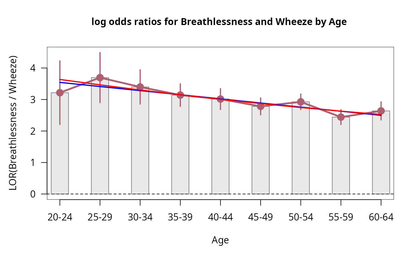
## 2 x 2 x k cases
data(CoalMiners, package = "vcd")
lor_CM <- loddsratio(CoalMiners)
plot(lor_CM)
lor_CM_df <- as.data.frame(lor_CM)

# fit linear models using WLS
age <- seq(20, 60, by = 5)
lmod <- lm(LOR ~ age, weights = 1 / ASE^2, data = lor_CM_df)
grid.lines(seq_along(age), fitted(lmod), gp = gpar(col = "blue", lwd = 2), default.units = "native")
qmod <- lm(LOR ~ poly(age, 2), weights = 1 / ASE^2, data = lor_CM_df)
grid.lines(seq_along(age), fitted(qmod), gp = gpar(col = "red", lwd = 2), default.units = "native")


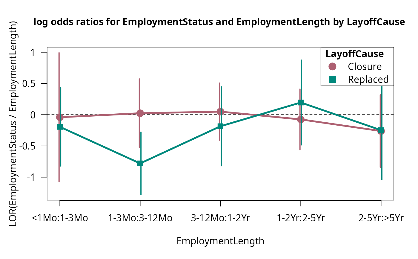
## 2 x k x 2
lor_Emp <-loddsratio(Employment)
plot(lor_Emp)


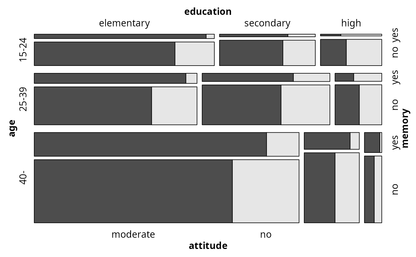
## 4 way tables 
data(Punishment, package = "vcd")
mosaic(attitude ~ age + education + memory, data = Punishment,
highlighting_direction="left", rep = c(attitude = FALSE))


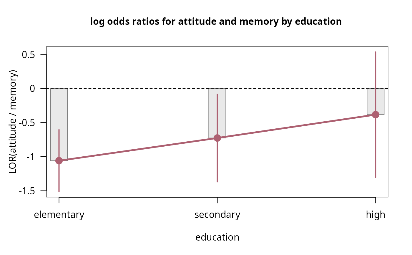
# visualize the log odds ratios, by education
plot(loddsratio(~ attitude + memory | education, data = Punishment))


# visualize the log odds ratios, by age
plot(loddsratio(~ attitude + memory | age, data = Punishment))


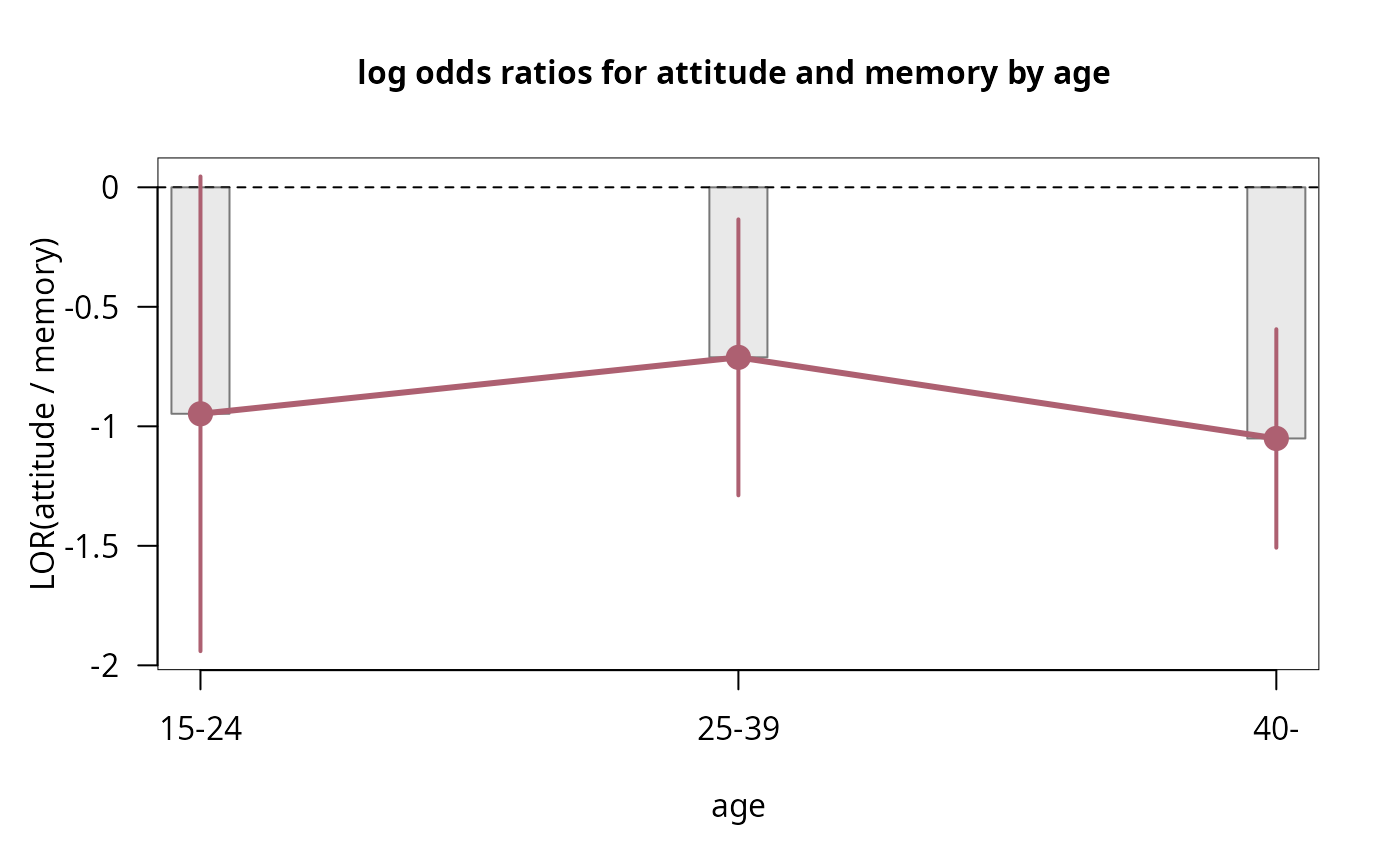
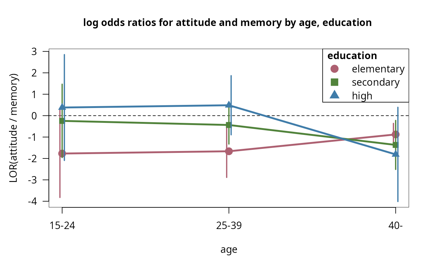
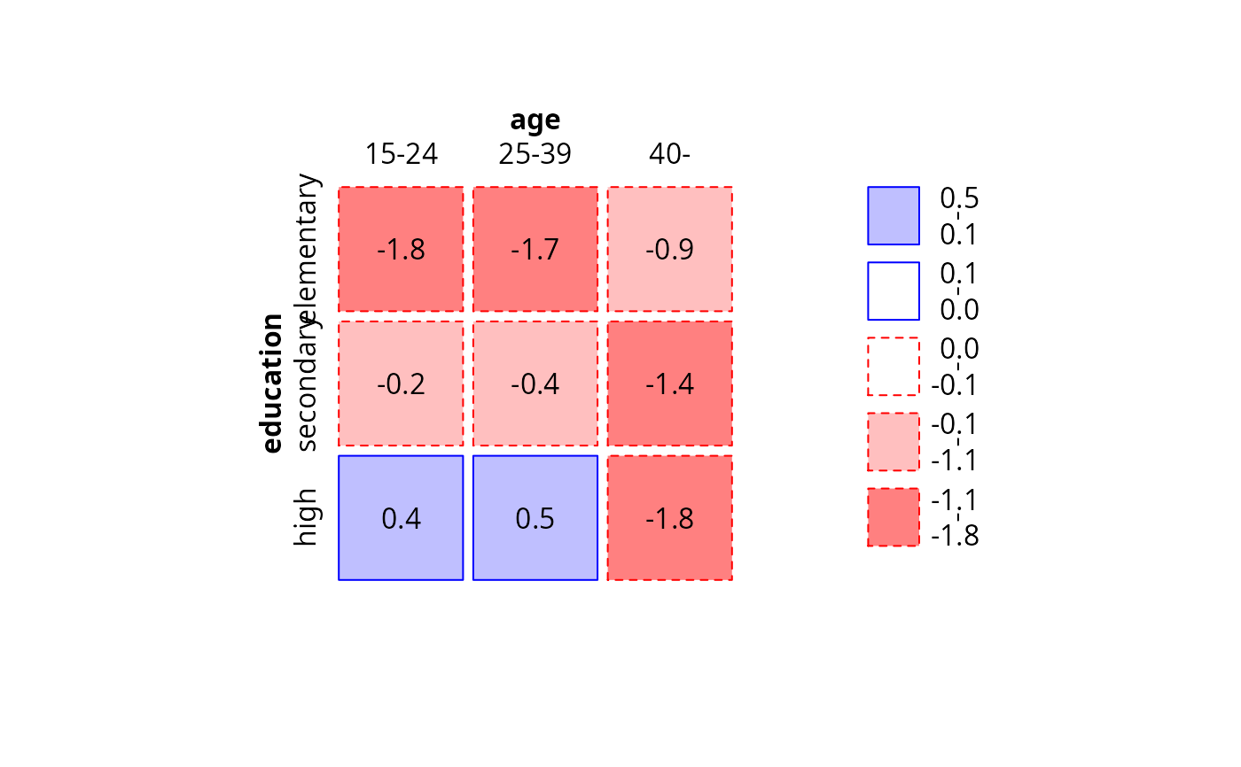
# visualize the log odds ratios, by age and education
plot(loddsratio(~ attitude + memory | age + education, data = Punishment))


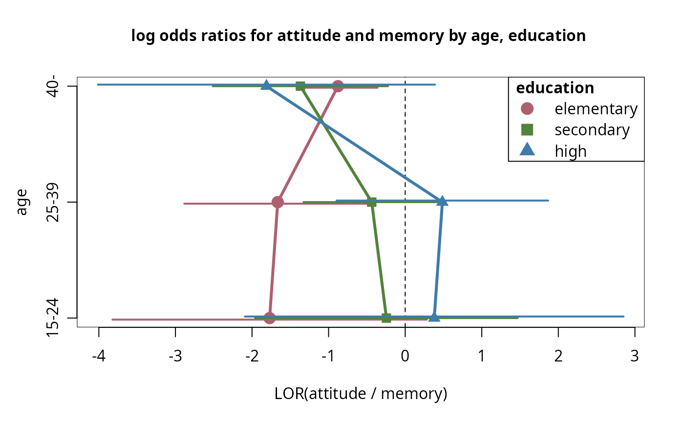
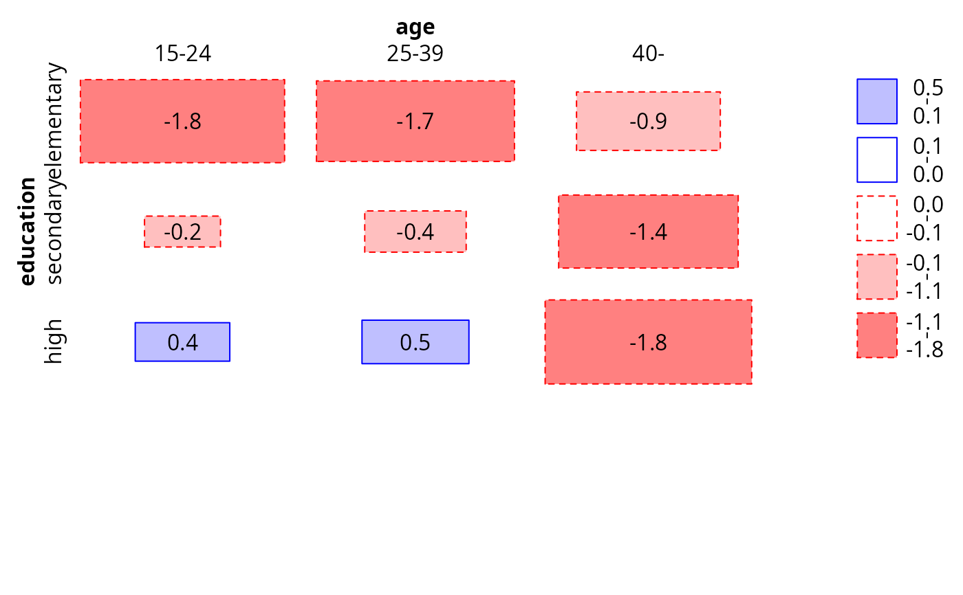
# same, transposed
plot(loddsratio(~ attitude + memory | age + education, data = Punishment), transpose = TRUE)


# alternative visualization methods
image(loddsratio(Freq ~ ., data = Punishment))

tile(loddsratio(Freq ~ ., data = Punishment))


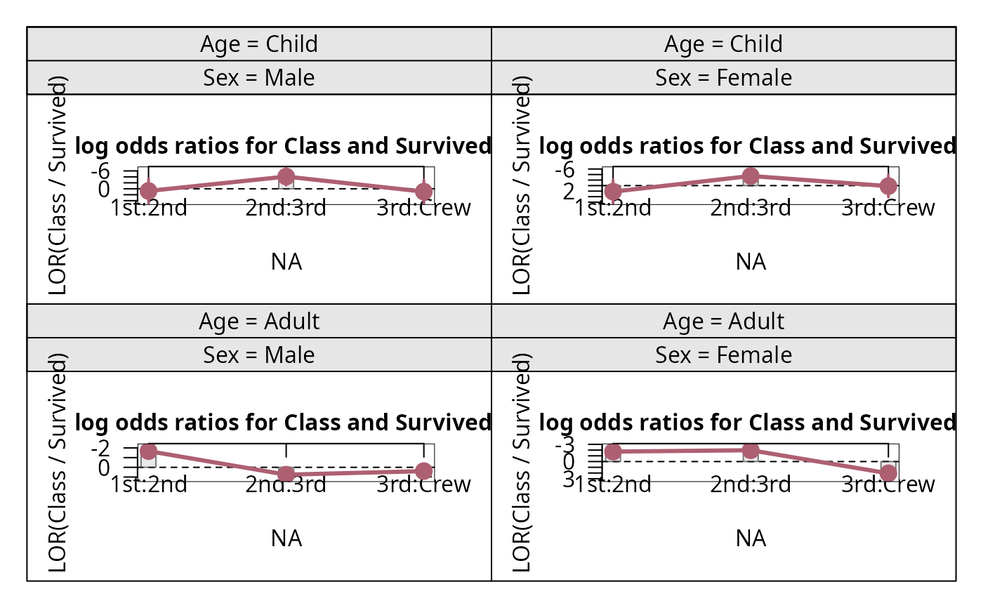
## cotabplots for more complex tables
cotabplot(Titanic, cond = c("Age","Sex"), panel = cotab_loddsratio)


cotabplot(Freq ~ opinion + grade + year | gender, data = JointSports, panel = cotab_loddsratio)

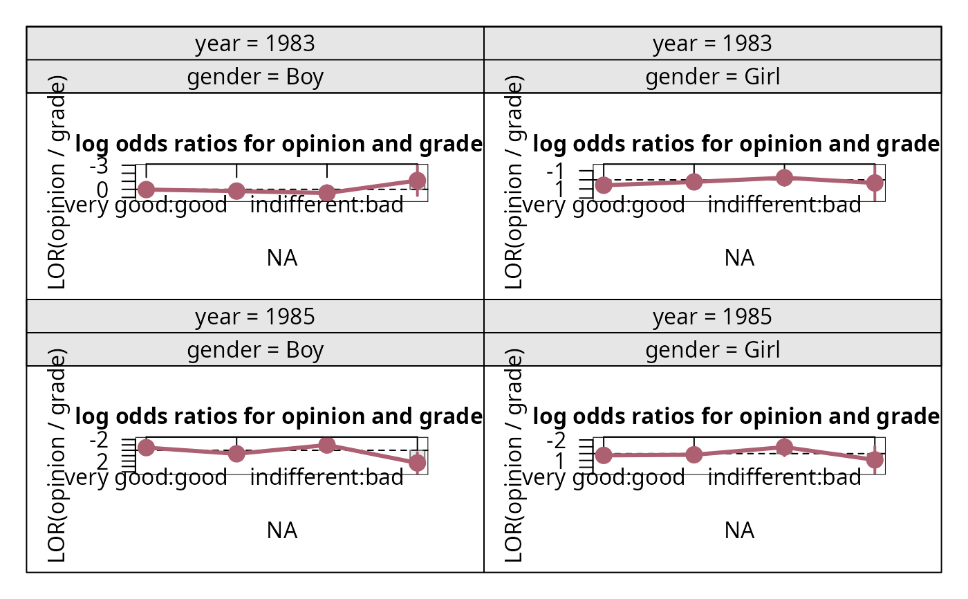
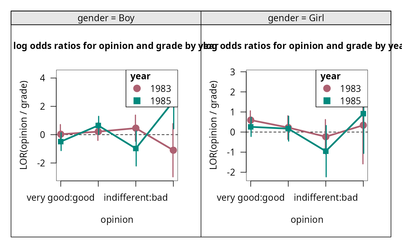cotabplot(Freq ~ opinion + grade | year + gender, data = JointSports, panel = cotab_loddsratio)