Panel-generating Functions for Contingency Table Coplots

Panel-generating functions visualizing contingency tables that can be passed to cotabplot.

cotab_mosaic(x = NULL, condvars = NULL, ...)
cotab_assoc(x = NULL, condvars = NULL, ylim = NULL, ...)
cotab_sieve(x = NULL, condvars = NULL, ...)
cotab_loddsratio(x = NULL, condvars = NULL, ...)
cotab_agreementplot(x = NULL, condvars = NULL, ...)
cotab_fourfold(x = NULL, condvars = NULL, ...)
cotab_coindep(x, condvars,
  test = c("doublemax", "maxchisq", "sumchisq"),
  level = NULL, n = 1000, interpolate = c(2, 4),
  h = NULL, c = NULL, l = NULL, lty = 1,
  type = c("mosaic", "assoc"), legend = FALSE, ylim = NULL, ...)

Arguments

x: a contingency tables in array form.
condvars: margin name(s) of the conditioning variables.
ylim: y-axis limits for assoc plot. By default this is computed from x.
test: character indicating which type of statistic should be used for assessing conditional independence.
level,n,h,c,l,lty,interpolate: variables controlling the HCL shading of the residuals, see shadings for more details.
type: character indicating which type of plot should be produced.
legend: logical. Should a legend be produced in each panel?
...: further arguments passed to the plotting function (such as mosaic or assoc or sieve respectively).

Details

These functions of class "panel_generator" are panel-generating functions for use with cotabplot, i.e., they return functions with the interface

panel(x, condlevels)

required for cotabplot. The functions produced by cotab_mosaic, cotab_assoc and cotab_sieve essentially only call co_table to produce the conditioned table and then call mosaic, assoc or sieve respectively with the arguments specified.

The function cotab_coindep is similar but additionally chooses an appropriate residual-based shading visualizing the associated conditional independence model. The conditional independence test is carried out via coindep_test and the shading is set up via shading_hcl.

A description of the underlying ideas is given in Zeileis, Meyer, Hornik (2005).

References

Meyer, D., Zeileis, A., and Hornik, K. (2006), The strucplot framework: Visualizing multi-way contingency tables with vcd. Journal of Statistical Software, 17(3), 1-48. doi:10.18637/jss.v017.i03 and available as vignette("strucplot").

Zeileis, A., Meyer, D., Hornik K. (2007), Residual-based shadings for visualizing (conditional) independence, Journal of Computational and Graphical Statistics, 16, 507–525.

Author

Achim Zeileis Achim.Zeileis@R-project.org

Examples

data("UCBAdmissions")

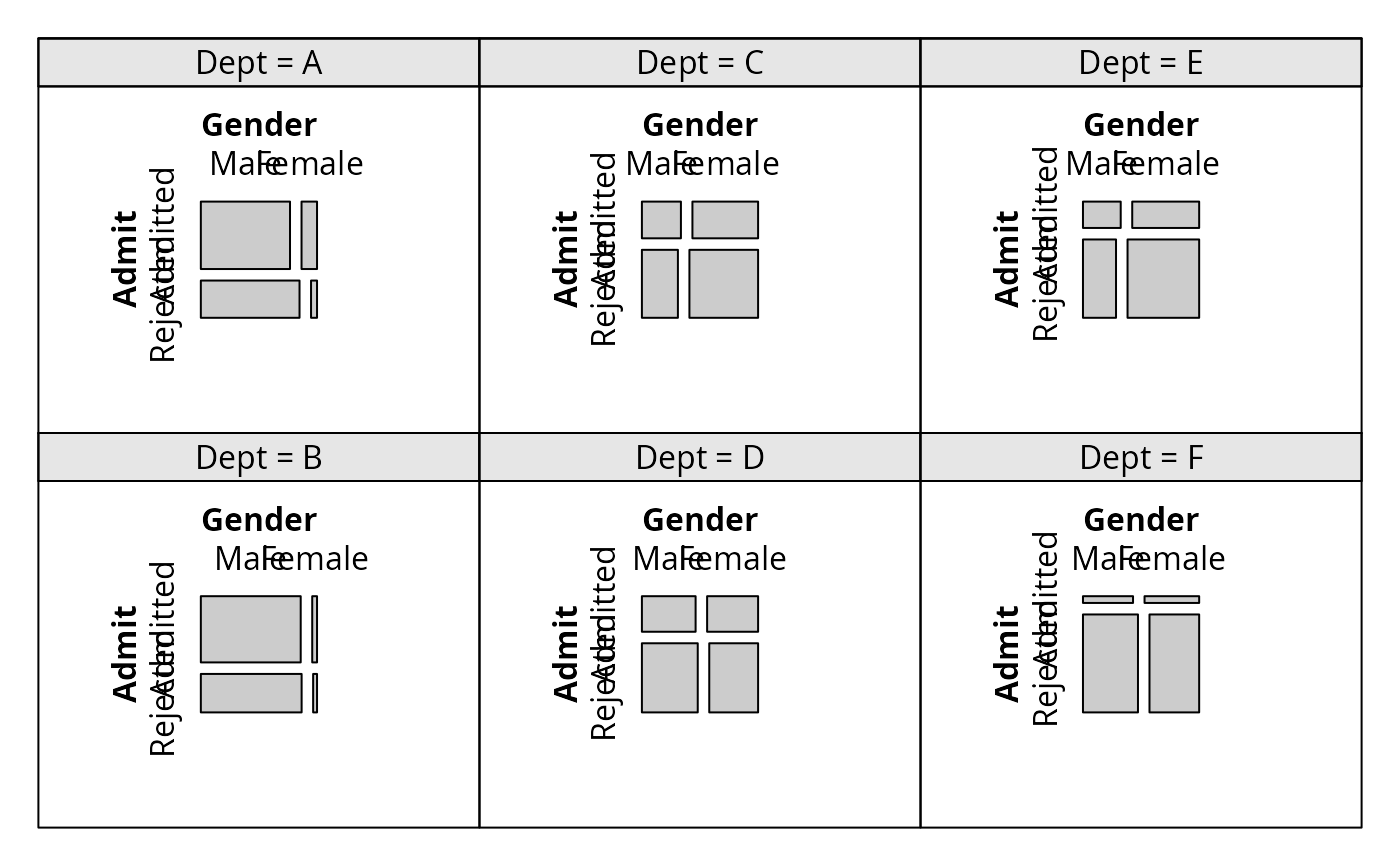
cotabplot(~ Admit + Gender | Dept, data = UCBAdmissions)

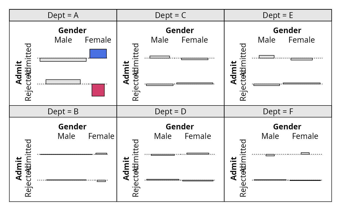
cotabplot(~ Admit + Gender | Dept, data = UCBAdmissions, panel = cotab_assoc)

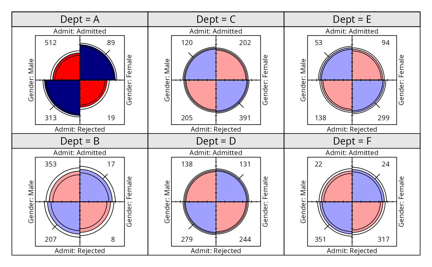
cotabplot(~ Admit + Gender | Dept, data = UCBAdmissions, panel = cotab_fourfold)


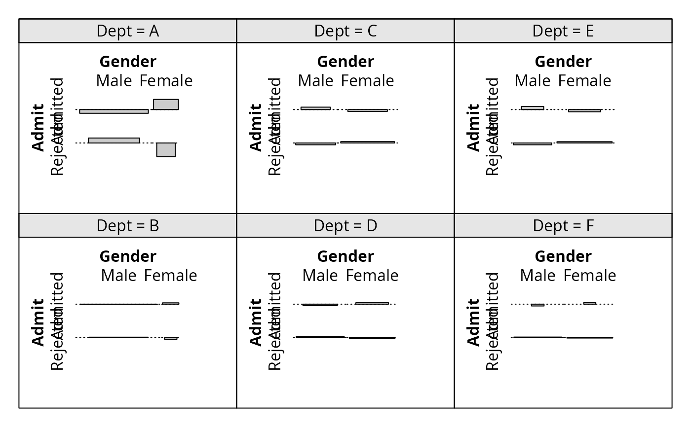
ucb <- cotab_coindep(UCBAdmissions, condvars = "Dept", type = "assoc",
                     n = 5000, margins = c(3, 1, 1, 3))
cotabplot(~ Admit + Gender | Dept, data = UCBAdmissions, panel = ucb)