Binary Regression Plot
binregplot.RdCreates a display of observed and fitted values for a binary regression model with one numeric predictor, conditioned by zero or many co-factors.
binreg_plot(model, main = NULL, xlab = NULL, ylab = NULL,
            xlim = NULL, ylim = NULL,
            pred_var = NULL, pred_range = c("data", "xlim"),
            group_vars = NULL, base_level = NULL, subset,
            type = c("response", "link"), conf_level = 0.95, delta = FALSE,
            pch = NULL, cex = 0.6, jitter_factor = 0.1,
            lwd = 5, lty = 1, point_size = 0, col_lines = NULL, col_bands = NULL,
            legend = TRUE, legend_pos = NULL, legend_inset = c(0, 0.1),
            legend_vgap = unit(0.5, "lines"),
            labels = FALSE, labels_pos = c("right", "left"),
            labels_just = c("left","center"), labels_offset = c(0.01, 0),
            gp_main = gpar(fontface = "bold", fontsize = 14),
            gp_legend_frame = gpar(lwd = 1, col = "black"),
            gp_legend_title = gpar(fontface = "bold"),
            newpage = TRUE, pop = FALSE, return_grob = FALSE)
grid_abline(a, b, ...)
Arguments
- model
a binary regression model fitted with
glm.- main
user-specified main title.
- xlab
x-axis label. Defaults to the name of the (first) numeric predictor.
- ylab
y-axis label. Defaults to the name of the response - within either 'P(...)' or 'logit(...)', depending on the response type.
- xlim
Range of the x-axis. Defaults to the range of the numeric predictor.
- ylim
Range of the y-axis. Defaults to the unit interval on probability scale or the fitted values range on the link scale, depending on
type.- pred_var
character string of length 1 giving the name of the numeric predictor. Defaults to the first one found in the data set.
- pred_range
"data","xlim", or a numeric vector. If"data", the numeric predictor corresponds to the observed values. If"xlim", 100 values are taken from the"xlim"range. A numeric vector will be interpreted as the values to be predicted.- group_vars
optional character string of conditioning variables. Defaults to all factors found in the data set, response excluded. If
FALSE, no variables are used for conditioning.- base_level
vector of length one. If the response is a vector, this specifies the base ('no effect') value of the response variable (e.g., "Placebo", 0, FALSE, etc.) and defaults to the first level for factor responses, or 0 for numeric/binary variables. This controls which observations will be plotted on the top or the bottom of the display. If the response is a matrix with success and failure column, this specifies the one to be interpreted as failure (default: 2), either as an integer, or as a string (
"success"or"failure"). The proportions of successes will be plotted as observed values.- subset
an optional vector specifying a subset of the data rows. The value is evaluated in the data environment, so expressions can be used to select the data (see examples).
- type
either "response" or "link" to select the scale of the fitted values. The y-axis will be adapted accordingly.
- conf_level
confidence level used for calculating confidence bands.
- delta
logical; indicates whether the delta method should be employed for calculating the limits of the confidence band or not (see details).
- pch
character or numeric vector of symbols used for plotting the (possibly conditioned) observed values, recycled as needed.
- cex
size of the plot symbols (in lines).
- jitter_factor
argument passed to
jitterused for the points representing the observed values.- lwd
Line width for the fitted values.
- lty
Line type for the fitted values.
- point_size
size of points for the fitted values in char units (default: 0, so no points are plotted).
- col_lines, col_bands
character vector specifying the colors of the fitted lines and confidence bands, by default chosen with
rainbow_hcl. The confidence bands are using alpha blending with alpha = 0.2.- legend
logical; if
TRUE(default), a legend is drawn.- legend_pos
numeric vector of length 2, specifying x and y coordinates of the legend, or a character string (e.g.,
"topleft","center"etc.). Defaults to"topleft"if the fitted curve's slope is positive, and"topright"else.- legend_inset
numeric vector or length 2 specifying the inset from the legend's x and y coordinates in npc units.
- legend_vgap
vertical space between the legend's line entries.
- labels
logical; if
TRUE, labels corresponding to the factor levels are plotted next to the fitted lines.- labels_pos
either
"right"or"left", determining on which side of the fitted lines (start or end) the labels should be placed.- labels_just
character vector of length 2, specifying the relative justification of the labels to their coordinates. See the documentation of the
justparameter ofgrid.textfor more details.- labels_offset
numeric vector of length 2, specifying the offset of the labels' coordinates in npc units.
- gp_main
object of class
"gpar"used for the main title.- gp_legend_frame
object of class
"gpar"used for the legend frame.- gp_legend_title
object of class
"gpar"used for the legend title.- newpage
logical; if
TRUE, the plot is drawn on a new page.- pop
logical; if
TRUE, all newly generated viewports are popped after plotting.- return_grob
logical. Should a snapshot of the display be returned as a grid grob?
- a
intercept; alternatively, a regression model from which coefficients can be extracted via
coef.- b
slope.
- ...
Further arguments passed to
grid.abline.
Details
The primary purpose of binreg_plot() is to visualize observed and
fitted values for binary regression models (like the logistic or probit
regression model) with one numeric predictor. If one or more
categorical predictors are used in the model, the fitted values are
conditioned on them, i.e. separate curves are drawn corresponding to
the factor level combinations. Thus, it shows a full-model plot, not a
conditional plot where several models would be fit to data subsets.
The implementation relies on objects returned by
glm, as it uses its "terms" and
"model" components.
The function tries to determine suitable values for the legend and/or labels, but depending on the data, this might require some tweaking.
By default, the limits of the confidence band are determined for the
linear predictor (i.e., on the link scale) and transformed to response
scale (if this is the chosen plot type) using the inverse link
function. If delta is TRUE, the limits
are determined on the response scale. Note that the resulting band using the
delta method is symmetric around the fitted mean,
but may exceed the unit interval (on the response scale) and
will be cut off.
grid_abline() is a simple convenience wrapper for
grid.abline with similar behavior than
abline in that it extracts coefficients from
a regression model, if given instead of the intercept a.
Value
if return_grob is TRUE, a grob object corresponding to
the plot. NULL (invisibly) else.
References
Michael Friendly (2000), Visualizing Categorical Data. SAS Institute, Cary, NC.
Examples
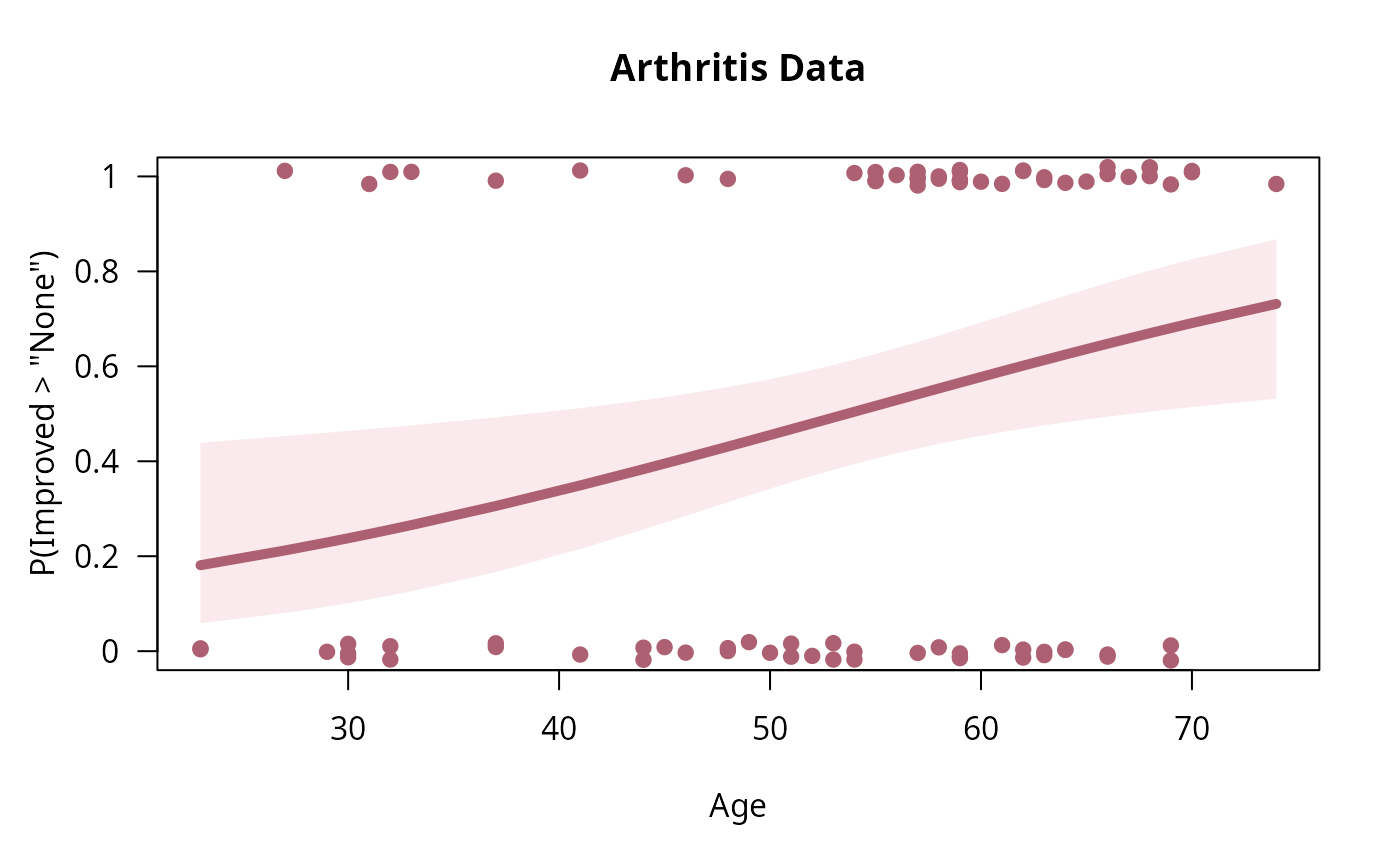
## Simple model with no conditioning variables
art.mod0 <- glm(Improved > "None" ~ Age, data = Arthritis, family = binomial)
binreg_plot(art.mod0, "Arthritis Data")
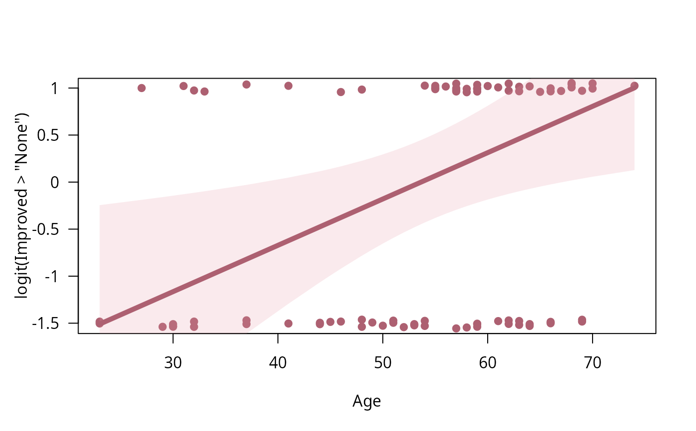
 binreg_plot(art.mod0, type = "link") ## logit scale
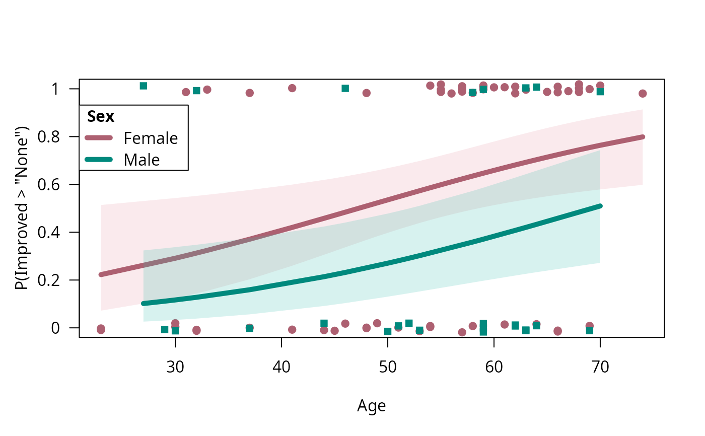
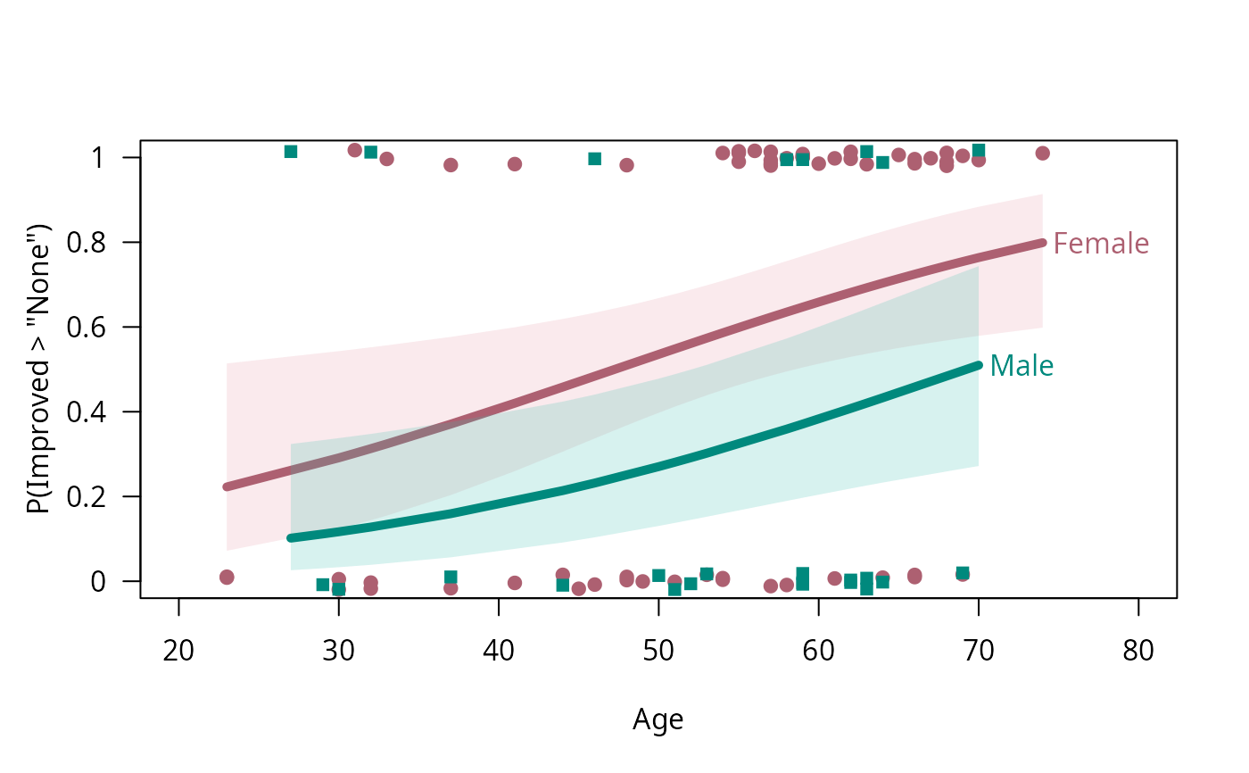
 ## one conditioning factor
art.mod1 <- update(art.mod0, . ~ . + Sex)
binreg_plot(art.mod1)
## one conditioning factor
art.mod1 <- update(art.mod0, . ~ . + Sex)
binreg_plot(art.mod1)
 binreg_plot(art.mod1, legend = FALSE, labels = TRUE, xlim = c(20, 80))
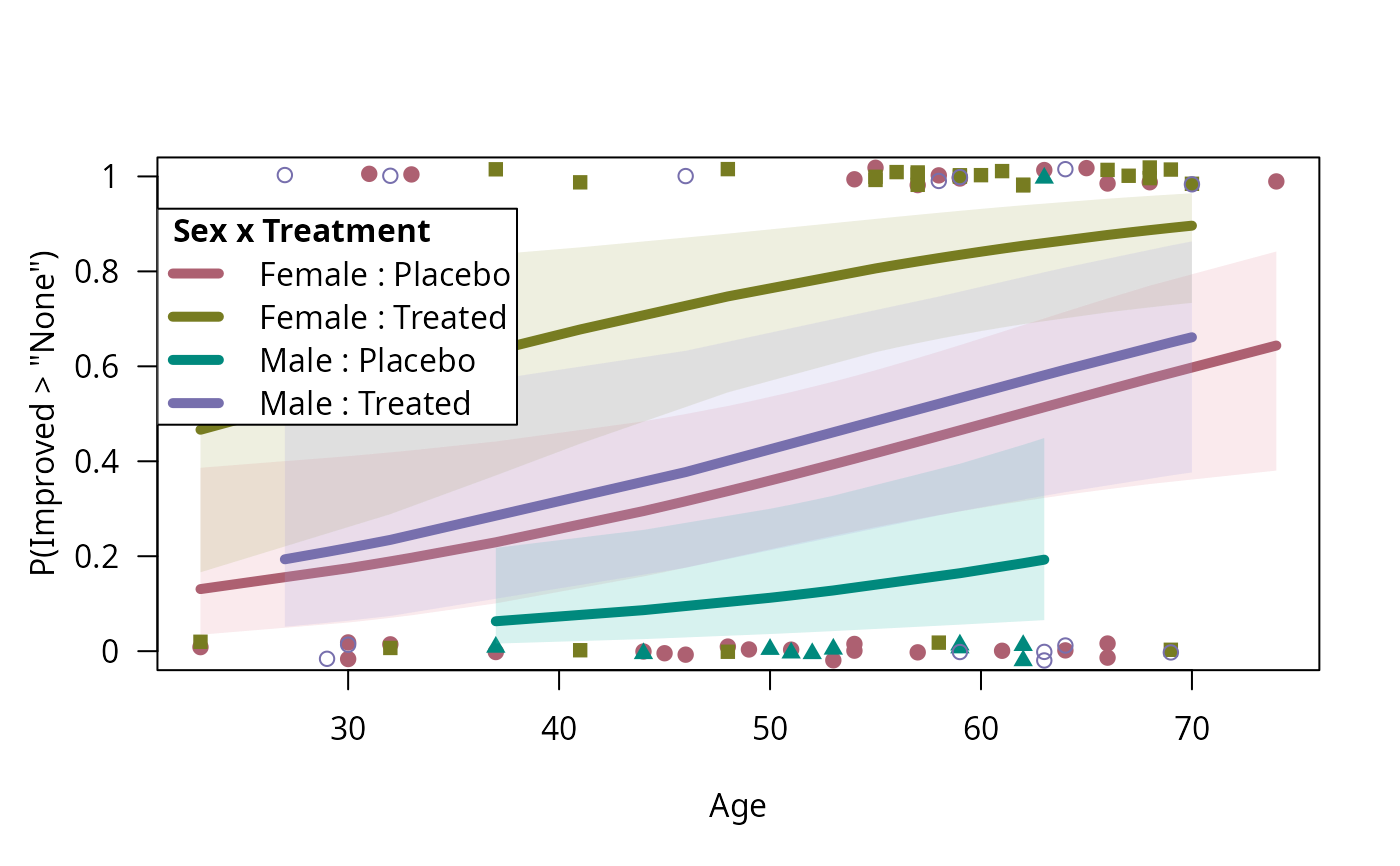
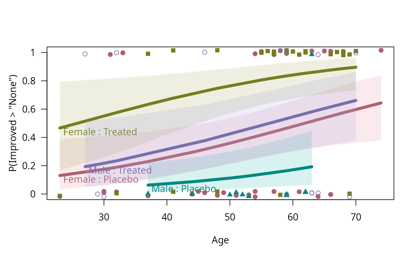
 ## two conditioning factors
art.mod2 <- update(art.mod1, . ~ . + Treatment)
binreg_plot(art.mod2)
## two conditioning factors
art.mod2 <- update(art.mod1, . ~ . + Treatment)
binreg_plot(art.mod2)
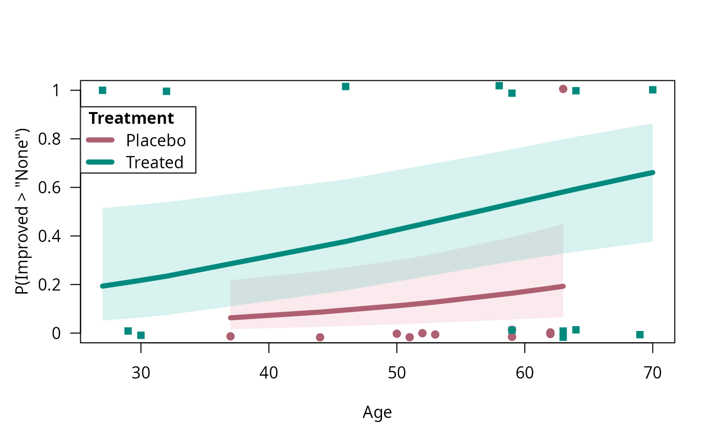
 binreg_plot(art.mod2, subset = Sex == "Male") ## subsetting
 ## some tweaking
binreg_plot(art.mod2, gp_legend_frame = gpar(col = NA, fill = "white"), col_bands = NA)
## some tweaking
binreg_plot(art.mod2, gp_legend_frame = gpar(col = NA, fill = "white"), col_bands = NA)
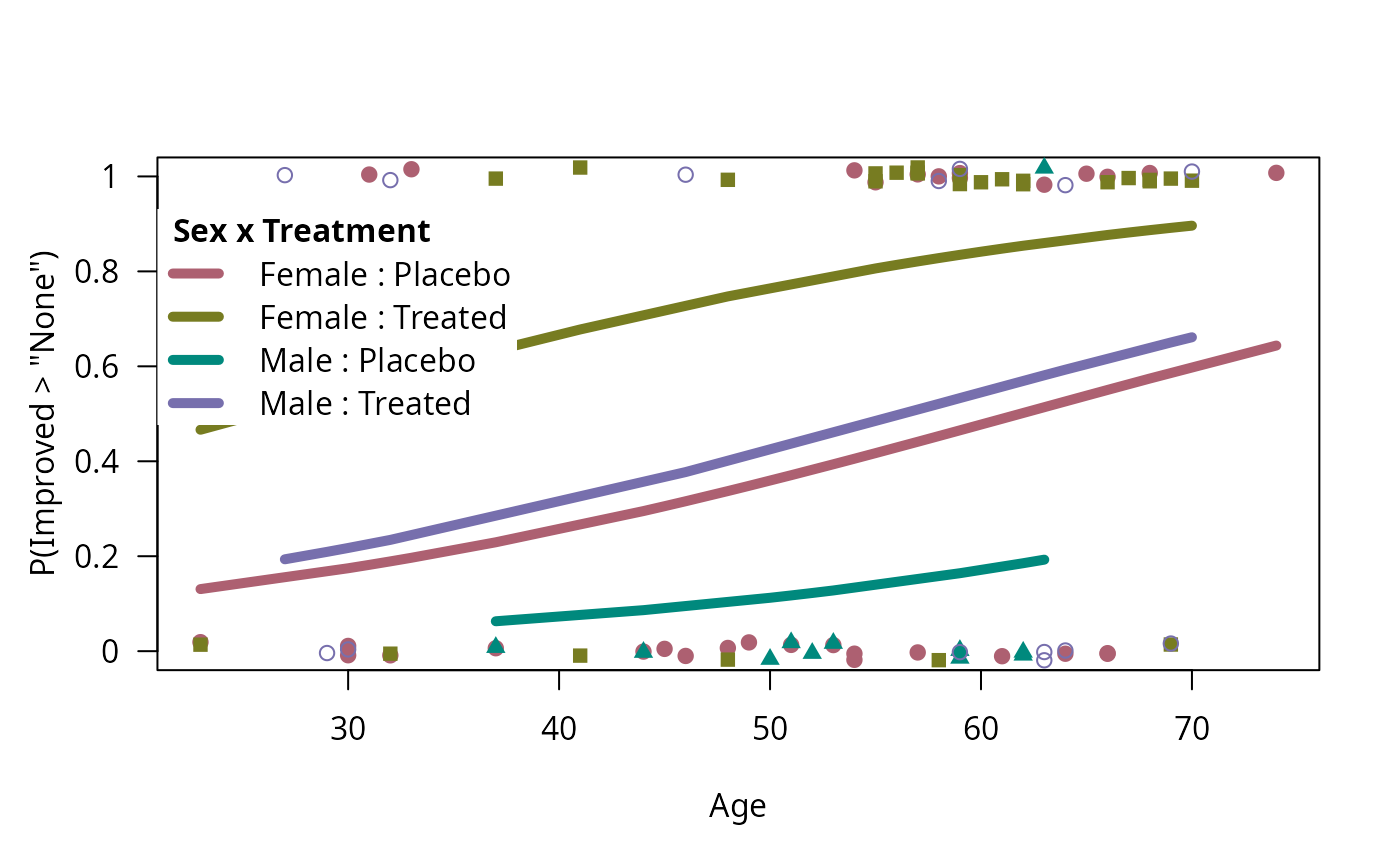 binreg_plot(art.mod2, legend = FALSE, labels = TRUE,
labels_pos = "left", labels_just = c("left", "top"))
binreg_plot(art.mod2, legend = FALSE, labels = TRUE,
labels_pos = "left", labels_just = c("left", "top"))
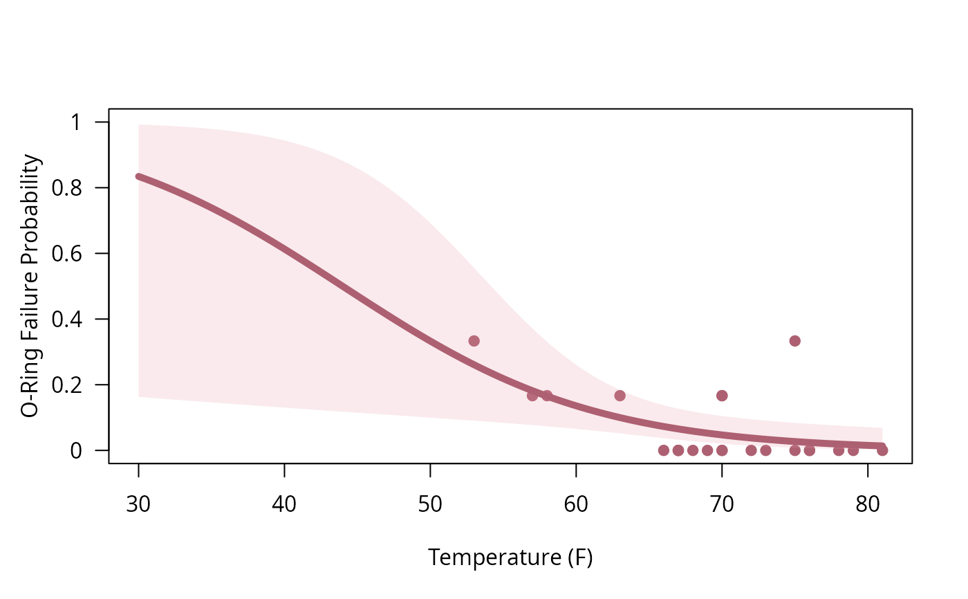
 ## model with grouped response data
shuttle.mod <- glm(cbind(nFailures, 6 - nFailures) ~ Temperature,
data = SpaceShuttle, na.action = na.exclude, family = binomial)
binreg_plot(shuttle.mod, xlim = c(30, 81), pred_range = "xlim",
ylab = "O-Ring Failure Probability", xlab = "Temperature (F)")
## model with grouped response data
shuttle.mod <- glm(cbind(nFailures, 6 - nFailures) ~ Temperature,
data = SpaceShuttle, na.action = na.exclude, family = binomial)
binreg_plot(shuttle.mod, xlim = c(30, 81), pred_range = "xlim",
ylab = "O-Ring Failure Probability", xlab = "Temperature (F)")