Bangdiwala's Observer Agreement Chart

Representation of a \(k \times k\) confusion matrix, where the observed and expected diagonal elements are represented by superposed black and white rectangles, respectively. The function also computes a statistic measuring the strength of agreement (relation of respective area sums).

# Default S3 method
agreementplot(x, reverse_y = TRUE, main = NULL,
              weights = c(1, 1 - 1/(ncol(x) - 1)^2), margins = par("mar"),
              newpage = TRUE, pop = TRUE, 
              xlab = names(dimnames(x))[2],
              ylab = names(dimnames(x))[1],
              xlab_rot = 0, xlab_just = "center",
              ylab_rot = 90, ylab_just = "center",
              fill_col = function(j) gray((1 - (weights[j]) ^ 2) ^ 0.5),
              line_col = "red", xscale = TRUE, yscale = TRUE,
              return_grob = FALSE,
              prefix = "", ...)
# S3 method for class 'formula'
agreementplot(formula, data = NULL, ..., subset)

Arguments

x: a confusion matrix, i.e., a table with equal-sized dimensions.
reverse_y: if TRUE, the y axis is reversed (i.e., the rectangles' positions correspond to the contingency table).
main: user-specified main title.
weights: vector of weights for successive larger observed areas, used in the agreement strength statistic, and also for the shading. The first element should be 1.
margins: vector of margins (see par).
newpage: logical; if TRUE, the plot is drawn on a new page.
pop: logical; if TRUE, all newly generated viewports are popped after plotting.
return_grob: logical. Should a snapshot of the display be returned as a grid grob?
xlab, ylab: labels of x- and y-axis.
xlab_rot, ylab_rot: rotation angle for the category labels.
xlab_just, ylab_just: justification for the category labels.
fill_col: a function, giving the fill colors used for exact and partial agreement
line_col: color used for the diagonal reference line
formula: a formula, such as y ~ x. For details, see xtabs.
data: a data frame (or list), or a contingency table from which the variables in formula should be taken.
subset: an optional vector specifying a subset of the rows in the data frame to be used for plotting.
xscale, yscale: logicals indicating whether the marginals should be added on the x-axis/y-axis, respectively.
prefix: character string used as prefix for the viewport name
...: further graphics parameters (see par).

Details

Weights can be specified to allow for partial agreement, taking into account contributions from off-diagonal cells. Partial agreement is typically represented in the display by lighter shading, as given by fill_col(j), corresponding to weights[j].

A weight vector of length 1 means strict agreement only, each additional element increases the maximum number of disagreement steps.

cotabplot can be used for stratified analyses (see examples).

Value

Invisibly returned, a list with components

Bangdiwala: the unweighted agreement strength statistic.
Bangdiwala_Weighted: the weighted statistic.
weights: the weight vector used.

References

Bangdiwala, S. I. (1988). The Agreement Chart. Department of Biostatistics, University of North Carolina at Chapel Hill, Institute of Statistics Mimeo Series No. 1859, https://repository.lib.ncsu.edu/bitstreams/fea554e9-8750-4f1a-8419-ee126ce1a790/download

Bangdiwala, S. I., Ana S. Haedo, Marcela L. Natal, and Andres Villaveces. The agreement chart as an alternative to the receiver-operating characteristic curve for diagnostic tests. Journal of Clinical Epidemiology, 61 (9), 866-874.

Michael Friendly (2000), Visualizing Categorical Data. SAS Institute, Cary, NC.

Author

David Meyer David.Meyer@R-project.org

Examples

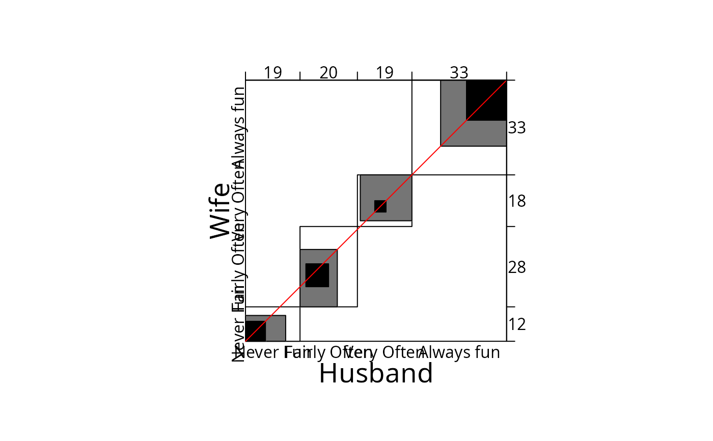
data("SexualFun")
agreementplot(t(SexualFun))


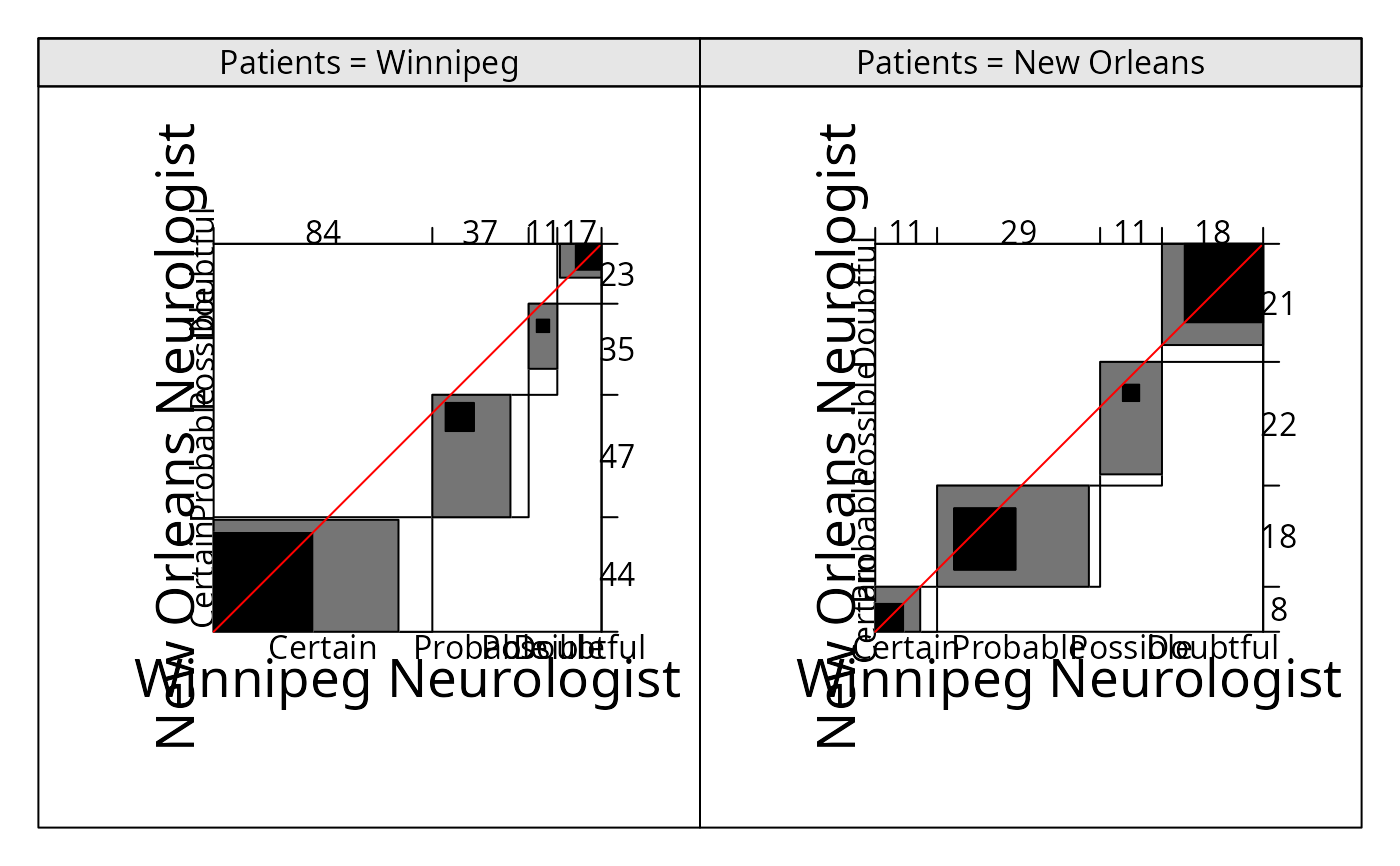
data("MSPatients")
if (FALSE) { # \dontrun{
## best visualized using a resized device, e.g. using:
## get(getOption("device"))(width = 12)
pushViewport(viewport(layout = grid.layout(ncol = 2)))
pushViewport(viewport(layout.pos.col = 1))
agreementplot(t(MSPatients[,,1]), main = "Winnipeg Patients",
              newpage = FALSE)
popViewport()
pushViewport(viewport(layout.pos.col = 2))
agreementplot(t(MSPatients[,,2]), main = "New Orleans Patients",
              newpage = FALSE)
popViewport(2)
dev.off()
} # }

## alternatively, use cotabplot:
cotabplot(MSPatients, panel = cotab_agreementplot)