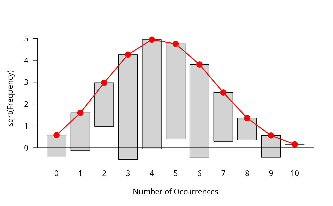
Women in Queues — WomenQueue • vcd

Data from Jinkinson & Slater (1981) and Hoaglin & Tukey (1985) reporting the frequency distribution of females in 100 queues of length 10 in a London Underground station.

data("WomenQueue")

Format

A 1-way table giving the number of women in 100 queues of length 10. The variable and its levels are

No	Name	Levels
1	nWomen	0, 1, ..., 10

References

D. C. Hoaglin & J. W. Tukey (1985), Checking the shape of discrete distributions. In D. C. Hoaglin, F. Mosteller, J. W. Tukey (eds.), Exploring Data Tables, Trends and Shapes, chapter 9. John Wiley & Sons, New York.

R. A. Jinkinson & M. Slater (1981), Critical discussion of a graphical method for identifying discrete distributions, The Statistician, 30, 239–248.

M. Friendly (2000), Visualizing Categorical Data. SAS Institute, Cary, NC.

Source

M. Friendly (2000), Visualizing Categorical Data, pages 19–20.

Examples

data("WomenQueue")
gf <- goodfit(WomenQueue, type = "binomial")
#> Warning: size was not given, taken as maximum count
summary(gf)
#> 
#> 	 Goodness-of-fit test for binomial distribution
#> 
#>                       X^2 df  P(> X^2)
#> Likelihood Ratio 8.650999  8 0.3725869
plot(gf)