Families in Saxony — Saxony • vcd

Data from Geissler, cited in Sokal & Rohlf (1969) and Lindsey (1995) on gender distributions in families in Saxony in the 19th century.

data("Saxony")

Format

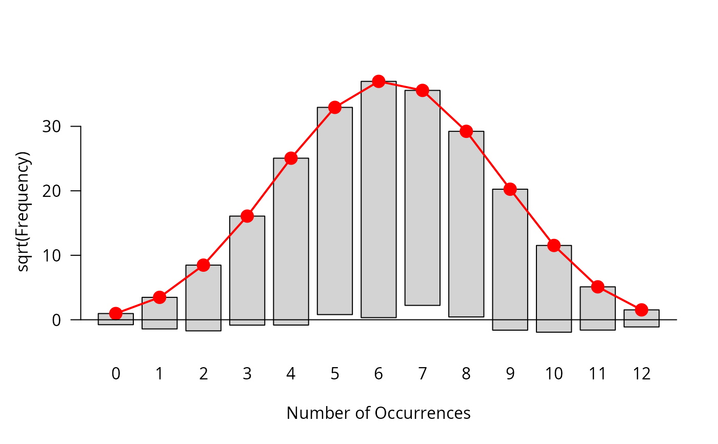
A 1-way table giving the number of male children in 6115 families of size 12. The variable and its levels are

No	Name	Levels
1	nMales	0, 1, ..., 12

References

J. K. Lindsey (1995), Analysis of Frequency and Count Data. Oxford University Press, Oxford, UK.

R. R. Sokal & F. J. Rohlf (1969), Biometry. The Principles and Practice of Statistics. W. H. Freeman, San Francisco, CA.

M. Friendly (2000), Visualizing Categorical Data. SAS Institute, Cary, NC.

Source

M. Friendly (2000), Visualizing Categorical Data, pages 40–42.

Examples

data("Saxony")
gf <- goodfit(Saxony, type = "binomial")
#> Warning: size was not given, taken as maximum count
summary(gf)
#> 
#> 	 Goodness-of-fit test for binomial distribution
#> 
#>                      X^2 df     P(> X^2)
#> Likelihood Ratio 97.0065 11 6.978187e-16
plot(gf)