Ord Plots
Ord_plot.RdOrd plots for diagnosing discrete distributions.
Ord_plot(obj, legend = TRUE, estimate = TRUE, tol = 0.1, type = NULL,
  xlim = NULL, ylim = NULL, xlab = "Number of occurrences",
  ylab = "Frequency ratio", main = "Ord plot", gp = gpar(cex = 0.5),
  lwd = c(2,2), lty=c(2,1), col=c("black", "red"),
  name = "Ord_plot", newpage = TRUE, pop = TRUE,
  return_grob = FALSE, ...)
Ord_estimate(x, type = NULL, tol = 0.1)
Arguments
- obj
either a vector of counts, a 1-way table of frequencies of counts or a data frame or matrix with frequencies in the first column and the corresponding counts in the second column.
- legend
logical. Should a legend be plotted?.
- estimate
logical. Should the distribution and its parameters be estimated from the data? See details.
- tol
tolerance for estimating the distribution. See details.
- type
a character string indicating the distribution, must be one of
"poisson","binomial","nbinomial"or"log-series"orNULL. In the latter case the distribution is estimated from the data. See details.- xlim
limits for the x axis.
- ylim
limits for the y axis.
- xlab
a label for the x axis.
- ylab
a label for the y axis.
- main
a title for the plot.
- gp
a
"gpar"object controlling the grid graphical parameters of the points.- lwd, lty
vectors of length 2, giving the line width and line type used for drawing the OLS line and the WLS lines.
- col
vector of length 2 giving the colors used for drawing the OLS and WLS lines.
- name
name of the plotting viewport.
- newpage
logical. Should
grid.newpagebe called before plotting?- pop
logical. Should the viewport created be popped?
- return_grob
logical. Should a snapshot of the display be returned as a grid grob?
- ...
further arguments passed to
grid.points.- x
a vector giving intercept and slope for the (fitted) line in the Ord plot.
Details
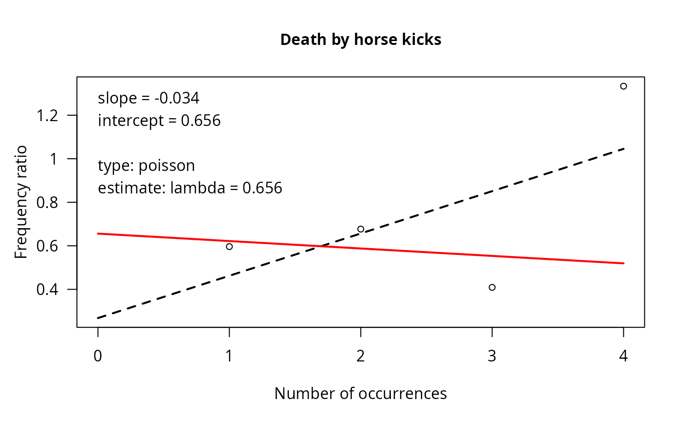
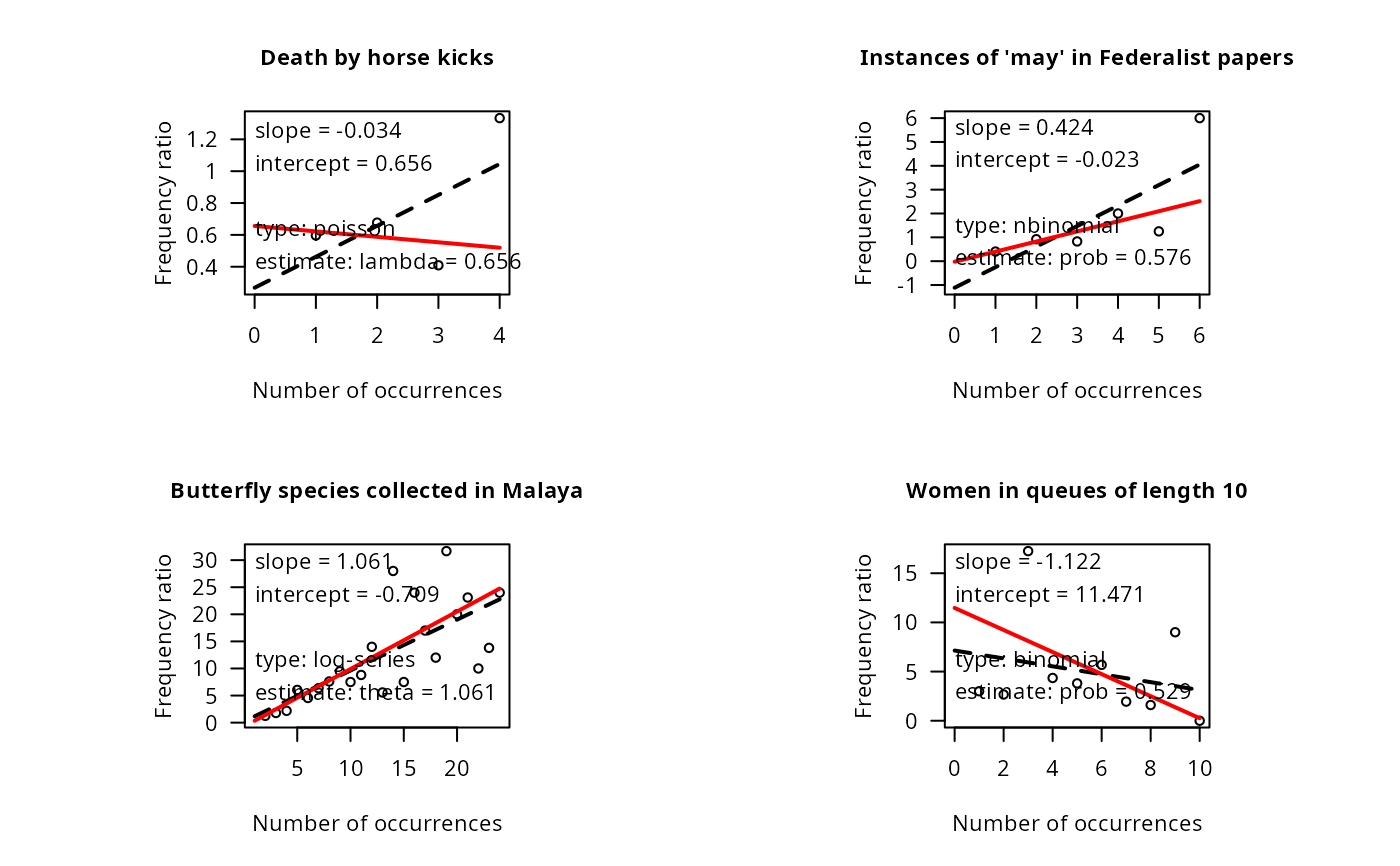
The Ord plot plots the number of occurrences against a certain frequency ratio (see Friendly (2000) for details) and should give a straight line if the data comes from a poisson, binomial, negative binomial or log-series distribution. The intercept and slope of this straight line conveys information about the underlying distribution.
Ord_plot fits a usual OLS line (black) and a weighted OLS line
(red). From the coefficients of the latter the distribution is
estimated by Ord_estimate as described in Table 2.10 in
Friendly (2000). To judge whether a coefficient is positive or
negative a tolerance given by tol is used. If none of the
distributions fits well, no parameters are estimated. Be careful with
the conclusions from Ord_estimate as it implements just some
simple heuristics!
Value
A vector giving the intercept and slope of the weighted OLS line.
References
J. K. Ord (1967), Graphical methods for a class of discrete distributions, Journal of the Royal Statistical Society, A 130, 232–238.
Michael Friendly (2000), Visualizing Categorical Data. SAS Institute, Cary, NC.
Examples
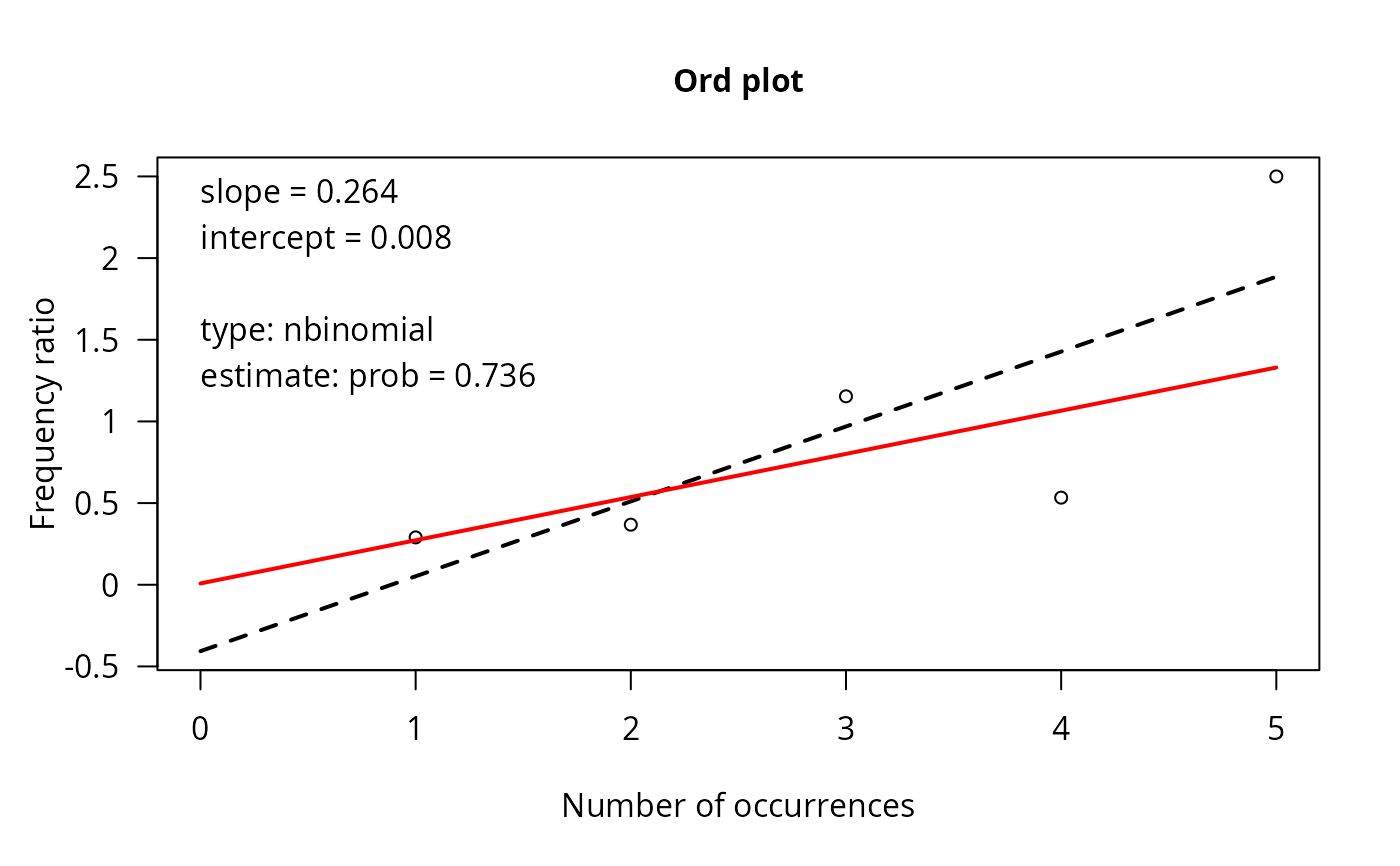
## Simulated data examples:
dummy <- rnbinom(1000, size = 1.5, prob = 0.8)
Ord_plot(dummy)
 ## Real data examples:
data("HorseKicks")
data("Federalist")
data("Butterfly")
data("WomenQueue")
if (FALSE) { # \dontrun{
grid.newpage()
pushViewport(viewport(layout = grid.layout(2, 2)))
pushViewport(viewport(layout.pos.col=1, layout.pos.row=1))
Ord_plot(HorseKicks, main = "Death by horse kicks", newpage = FALSE)
popViewport()
pushViewport(viewport(layout.pos.col=1, layout.pos.row=2))
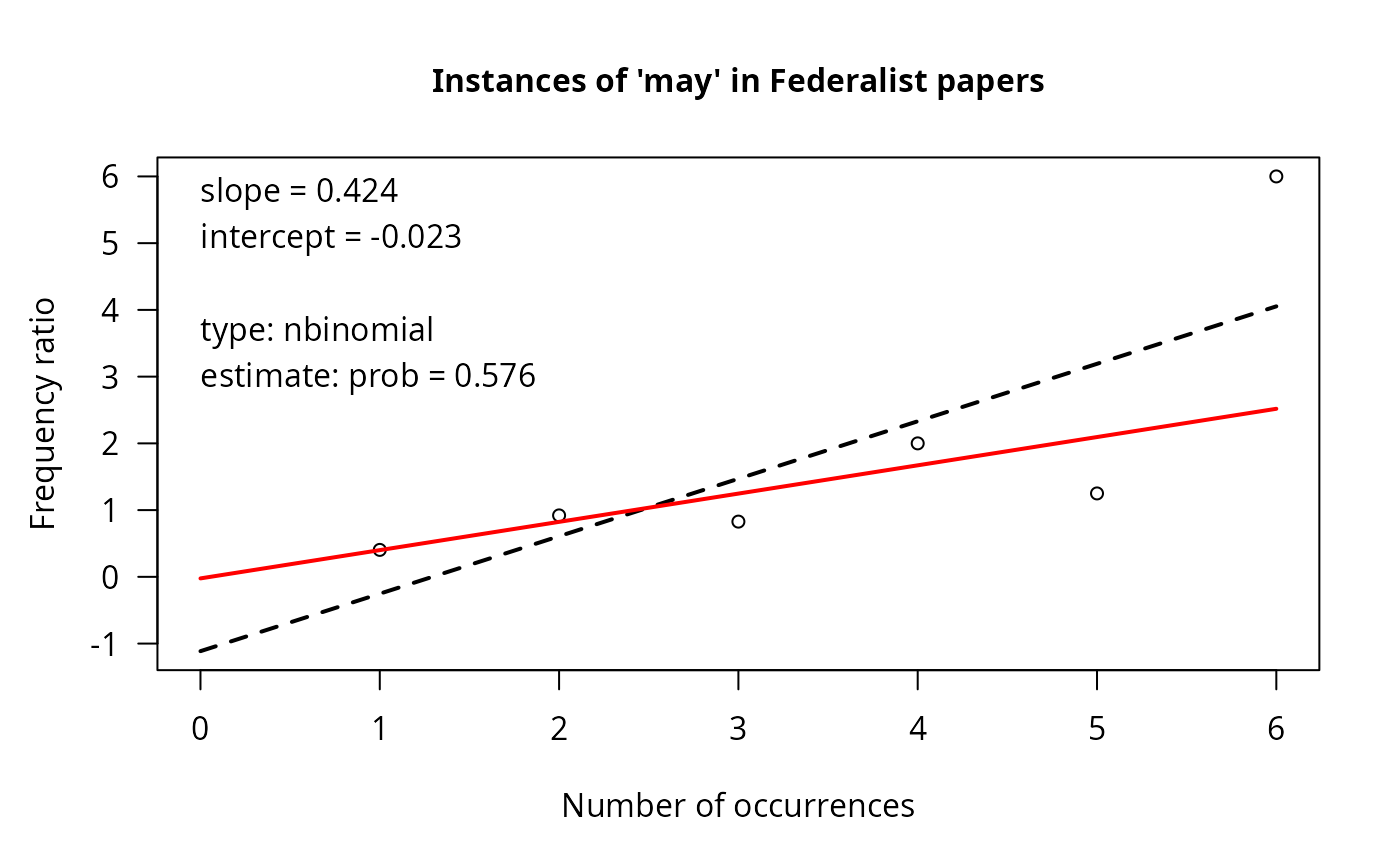
Ord_plot(Federalist, main = "Instances of 'may' in Federalist papers", newpage = FALSE)
popViewport()
pushViewport(viewport(layout.pos.col=2, layout.pos.row=1))
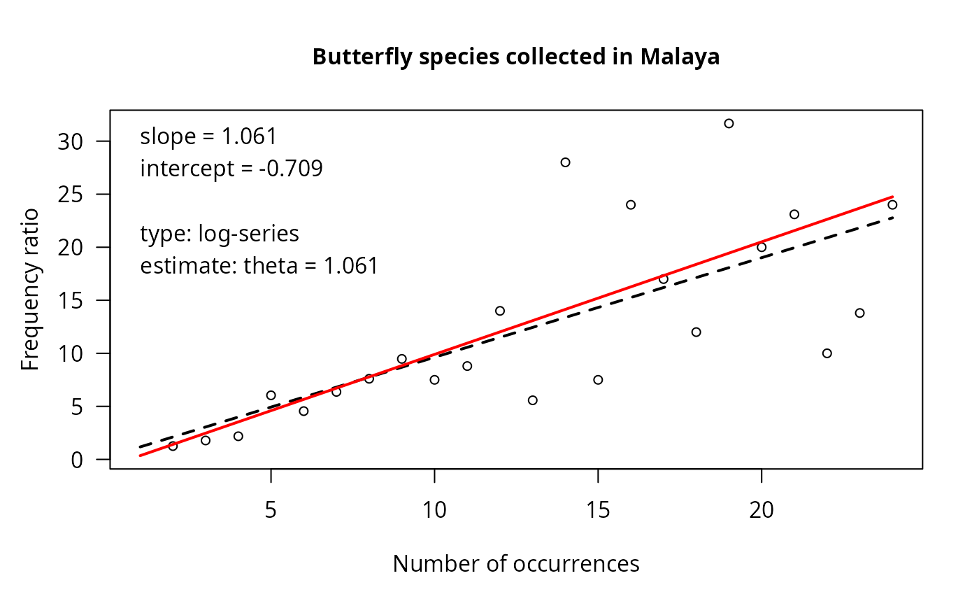
Ord_plot(Butterfly, main = "Butterfly species collected in Malaya", newpage = FALSE)
popViewport()
pushViewport(viewport(layout.pos.col=2, layout.pos.row=2))
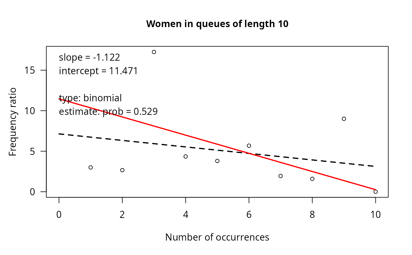
Ord_plot(WomenQueue, main = "Women in queues of length 10", newpage = FALSE)
popViewport(2)
} # }
## same
mplot(
Ord_plot(HorseKicks, return_grob = TRUE, main = "Death by horse kicks"),
Ord_plot(Federalist, return_grob = TRUE, main = "Instances of 'may' in Federalist papers"),
Ord_plot(Butterfly, return_grob = TRUE, main = "Butterfly species collected in Malaya"),
Ord_plot(WomenQueue, return_grob = TRUE, main = "Women in queues of length 10")
)
## Real data examples:
data("HorseKicks")
data("Federalist")
data("Butterfly")
data("WomenQueue")
if (FALSE) { # \dontrun{
grid.newpage()
pushViewport(viewport(layout = grid.layout(2, 2)))
pushViewport(viewport(layout.pos.col=1, layout.pos.row=1))
Ord_plot(HorseKicks, main = "Death by horse kicks", newpage = FALSE)
popViewport()
pushViewport(viewport(layout.pos.col=1, layout.pos.row=2))
Ord_plot(Federalist, main = "Instances of 'may' in Federalist papers", newpage = FALSE)
popViewport()
pushViewport(viewport(layout.pos.col=2, layout.pos.row=1))
Ord_plot(Butterfly, main = "Butterfly species collected in Malaya", newpage = FALSE)
popViewport()
pushViewport(viewport(layout.pos.col=2, layout.pos.row=2))
Ord_plot(WomenQueue, main = "Women in queues of length 10", newpage = FALSE)
popViewport(2)
} # }
## same
mplot(
Ord_plot(HorseKicks, return_grob = TRUE, main = "Death by horse kicks"),
Ord_plot(Federalist, return_grob = TRUE, main = "Instances of 'may' in Federalist papers"),
Ord_plot(Butterfly, return_grob = TRUE, main = "Butterfly species collected in Malaya"),
Ord_plot(WomenQueue, return_grob = TRUE, main = "Women in queues of length 10")
)