Breathlessness and Wheeze in Coal Miners
CoalMiners.RdData from Ashford & Sowden (1970) given by Agresti (1990) on the association between two pulmonary conditions, breathlessness and wheeze, in a large sample of coal miners who were smokers with no radiological evidence of pneumoconlosis, aged between 20–64 when examined. This data is frequently used as an example of fitting models for bivariate, binary responses.
data("CoalMiners")Format
A 3-dimensional table of size 2 x 2 x 9 resulting from cross-tabulating variables for 18,282 coal miners. The variables and their levels are as follows:
| No | Name | Levels |
| 1 | Breathlessness | B, NoB |
| 2 | Wheeze | W, NoW |
| 3 | Age | 20-24, 25-29, 30-34, ..., 60-64 |
Details
In an earlier version of this data set, the first group, aged 20-24, was inadvertently omitted from this data table and the breathlessness variable was called wheeze and vice versa.
References
A. Agresti (1990), Categorical Data Analysis. Wiley-Interscience, New York, Table 7.11, p. 237
J. R. Ashford and R. D. Sowdon (1970), Multivariate probit analysis, Biometrics, 26, 535–546.
M. Friendly (2000), Visualizing Categorical Data. SAS Institute, Cary, NC.
Source
Michael Friendly (2000), Visualizing Categorical Data, pages 82–83, 319–322.
Examples
data("CoalMiners")
ftable(CoalMiners, row.vars = 3)
#> Breathlessness B NoB
#> Wheeze W NoW W NoW
#> Age
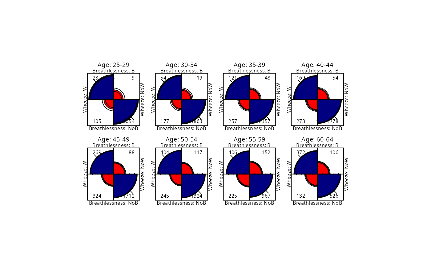
#> 20-24 9 7 95 1841
#> 25-29 23 9 105 1654
#> 30-34 54 19 177 1863
#> 35-39 121 48 257 2357
#> 40-44 169 54 273 1778
#> 45-49 269 88 324 1712
#> 50-54 404 117 245 1324
#> 55-59 406 152 225 967
#> 60-64 372 106 132 526
## Fourfold display, both margins equated
fourfold(CoalMiners[,,2:9], mfcol = c(2,4))
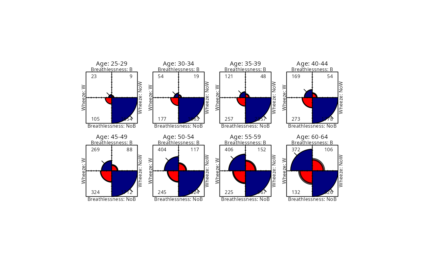
 ## Fourfold display, strata equated
fourfold(CoalMiners[,,2:9], std = "ind.max", mfcol = c(2,4))
## Fourfold display, strata equated
fourfold(CoalMiners[,,2:9], std = "ind.max", mfcol = c(2,4))
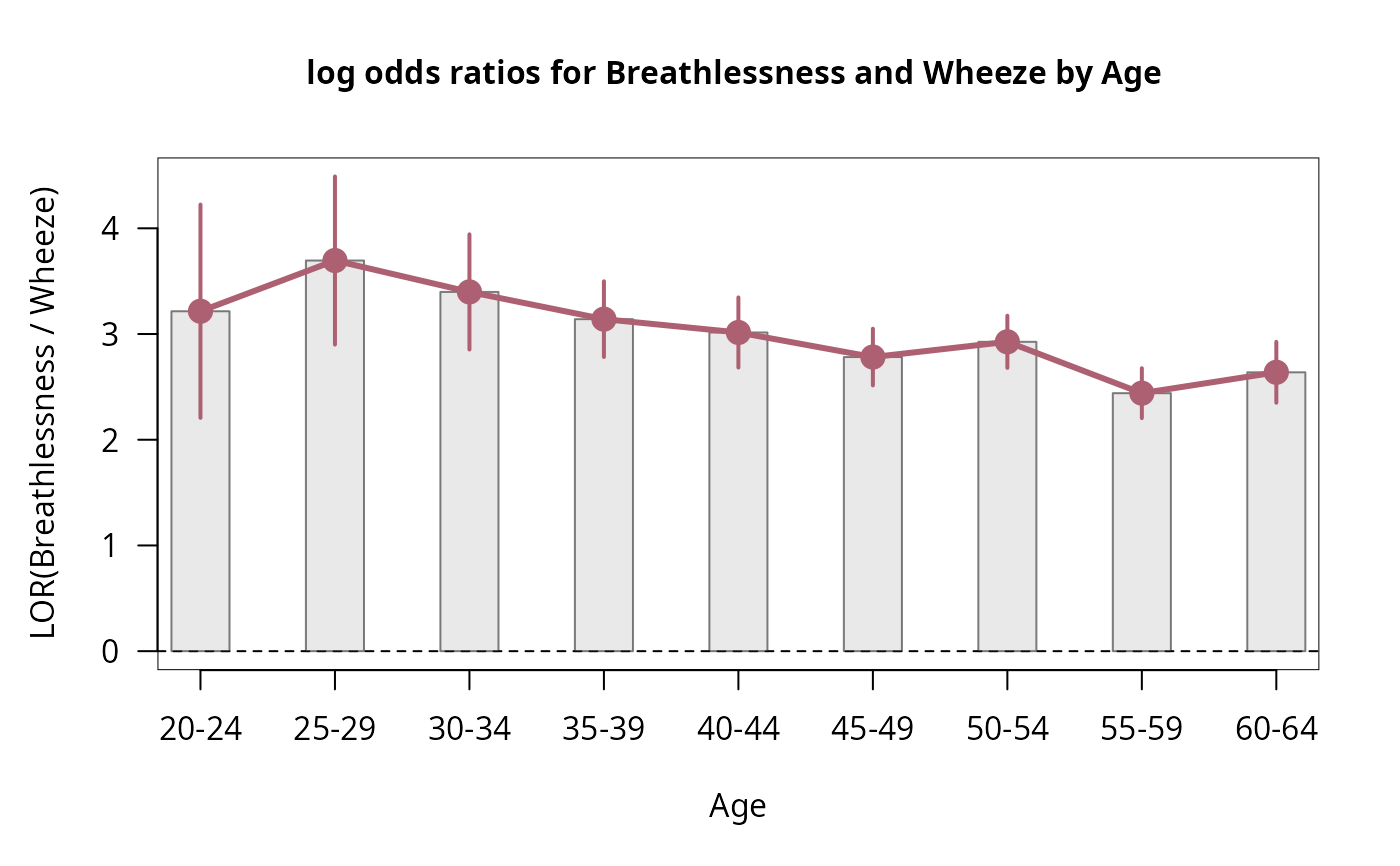
 ## Log Odds Ratio Plot
lor_CM <- loddsratio(CoalMiners)
summary(lor_CM)
#>
#> z test of coefficients:
#>
#> Estimate Std. Error z value Pr(>|z|)
#> 20-24 3.21550 0.51482 6.2459 4.214e-10 ***
#> 25-29 3.69526 0.40585 9.1049 < 2.2e-16 ***
#> 30-34 3.39834 0.27809 12.2201 < 2.2e-16 ***
#> 35-39 3.14066 0.18279 17.1815 < 2.2e-16 ***
#> 40-44 3.01469 0.16930 17.8072 < 2.2e-16 ***
#> 45-49 2.78205 0.13694 20.3163 < 2.2e-16 ***
#> 50-54 2.92640 0.12593 23.2377 < 2.2e-16 ***
#> 55-59 2.44057 0.12050 20.2535 < 2.2e-16 ***
#> 60-64 2.63795 0.14697 17.9494 < 2.2e-16 ***
#> ---
#> Signif. codes: 0 ‘***’ 0.001 ‘**’ 0.01 ‘*’ 0.05 ‘.’ 0.1 ‘ ’ 1
#>
plot(lor_CM)
lor_CM_df <- as.data.frame(lor_CM)
# fit linear models using WLS
age <- seq(20, 60, by = 5)
lmod <- lm(LOR ~ age, weights = 1 / ASE^2, data = lor_CM_df)
grid.lines(age, fitted(lmod), gp = gpar(col = "blue"))
qmod <- lm(LOR ~ poly(age, 2), weights = 1 / ASE^2, data = lor_CM_df)
grid.lines(age, fitted(qmod), gp = gpar(col = "red"))
## Log Odds Ratio Plot
lor_CM <- loddsratio(CoalMiners)
summary(lor_CM)
#>
#> z test of coefficients:
#>
#> Estimate Std. Error z value Pr(>|z|)
#> 20-24 3.21550 0.51482 6.2459 4.214e-10 ***
#> 25-29 3.69526 0.40585 9.1049 < 2.2e-16 ***
#> 30-34 3.39834 0.27809 12.2201 < 2.2e-16 ***
#> 35-39 3.14066 0.18279 17.1815 < 2.2e-16 ***
#> 40-44 3.01469 0.16930 17.8072 < 2.2e-16 ***
#> 45-49 2.78205 0.13694 20.3163 < 2.2e-16 ***
#> 50-54 2.92640 0.12593 23.2377 < 2.2e-16 ***
#> 55-59 2.44057 0.12050 20.2535 < 2.2e-16 ***
#> 60-64 2.63795 0.14697 17.9494 < 2.2e-16 ***
#> ---
#> Signif. codes: 0 ‘***’ 0.001 ‘**’ 0.01 ‘*’ 0.05 ‘.’ 0.1 ‘ ’ 1
#>
plot(lor_CM)
lor_CM_df <- as.data.frame(lor_CM)
# fit linear models using WLS
age <- seq(20, 60, by = 5)
lmod <- lm(LOR ~ age, weights = 1 / ASE^2, data = lor_CM_df)
grid.lines(age, fitted(lmod), gp = gpar(col = "blue"))
qmod <- lm(LOR ~ poly(age, 2), weights = 1 / ASE^2, data = lor_CM_df)
grid.lines(age, fitted(qmod), gp = gpar(col = "red"))