Fit GARCH Models to Time Series
garch.RdFit a Generalized Autoregressive Conditional Heteroscedastic GARCH(p, q) time series model to the data by computing the maximum-likelihood estimates of the conditionally normal model.
Usage
garch(x, order = c(1, 1), series = NULL, control = garch.control(...), ...)

garch.control(maxiter = 200, trace = TRUE, start = NULL,
  grad = c("analytical","numerical"), abstol = max(1e-20, .Machine$double.eps^2),
  reltol = max(1e-10, .Machine$double.eps^(2/3)), xtol = sqrt(.Machine$double.eps),
  falsetol = 1e2 * .Machine$double.eps, ...)
Arguments
- x
a numeric vector or time series.
- order
a two dimensional integer vector giving the orders of the model to fit.
order[2]corresponds to the ARCH part andorder[1]to the GARCH part.- series
name for the series. Defaults to
deparse(substitute(x)).- control
a list of control parameters as set up by
garch.control.- maxiter
gives the maximum number of log-likelihood function evaluations
maxiterand the maximum number of iterations2*maxiterthe optimizer is allowed to compute.- trace
logical. Trace optimizer output?
- start
If given this numeric vector is used as the initial estimate of the GARCH coefficients. Default initialization is to set the GARCH parameters to slightly positive values and to initialize the intercept such that the unconditional variance of the initial GARCH is equal to the variance of
x.- grad
character indicating whether analytical gradients or a numerical approximation is used for the optimization.
- abstol
absolute function convergence tolerance.
- reltol
relative function convergence tolerance.
- xtol
coefficient-convergence tolerance.
- falsetol
false convergence tolerance.
- ...
additional arguments for
qrwhen computing the asymptotic covariance matrix.
Details
garch uses a Quasi-Newton optimizer to find the maximum
likelihood estimates of the conditionally normal model. The first
max(p, q) values are assumed to be fixed. The optimizer uses a hessian
approximation computed from the BFGS update. Only a Cholesky factor
of the Hessian approximation is stored. For more details see Dennis
et al. (1981), Dennis and Mei (1979), Dennis and More (1977), and
Goldfarb (1976). The gradient is either computed analytically or
using a numerical approximation.
Value
A list of class "garch" with the following elements:
- order
the order of the fitted model.
- coef
estimated GARCH coefficients for the fitted model.
- n.likeli
the negative log-likelihood function evaluated at the coefficient estimates (apart from some constant).
- n.used
the number of observations of
x.- residuals
the series of residuals.
- fitted.values
the bivariate series of conditional standard deviation predictions for
x.- series
the name of the series
x.- frequency
the frequency of the series
x.- call
the call of the
garchfunction.- vcov
outer product of gradient estimate of the asymptotic-theory covariance matrix for the coefficient estimates.
References
A. K. Bera and M. L. Higgins (1993): ARCH Models: Properties, Estimation and Testing. J. Economic Surveys 7 305–362. doi:10.1111/j.1467-6419.1993.tb00170.x .
T. Bollerslev (1986): Generalized Autoregressive Conditional Heteroscedasticity. Journal of Econometrics 31, 307–327. doi:10.1016/0304-4076(86)90063-1 .
R. F. Engle (1982): Autoregressive Conditional Heteroscedasticity with Estimates of the Variance of United Kingdom Inflation. Econometrica 50, 987–1008. doi:10.1093/oso/9780198774310.003.0001 .
J. E. Dennis, D. M. Gay, and R. E. Welsch (1981): Algorithm 573 — An Adaptive Nonlinear Least-Squares Algorithm. ACM Transactions on Mathematical Software 7, 369–383. doi:10.1145/355958.355966 .
J. E. Dennis and H. H. W. Mei (1979): Two New Unconstrained Optimization Algorithms which use Function and Gradient Values. J. Optim. Theory Applic. 28, 453–482. doi:10.1007/BF00932218 .
J. E. Dennis and J. J. More (1977): Quasi-Newton Methods, Motivation and Theory. SIAM Rev. 19, 46–89. doi:10.1137/1019005 .
D. Goldfarb (1976): Factorized Variable Metric Methods for Unconstrained Optimization. Math. Comput. 30, 796–811. doi:10.2307/2005399 .
See also
summary.garch for summarizing GARCH model fits;
garch-methods for further methods.
Examples
n <- 1100
a <- c(0.1, 0.5, 0.2) # ARCH(2) coefficients
e <- rnorm(n)
x <- double(n)
x[1:2] <- rnorm(2, sd = sqrt(a[1]/(1.0-a[2]-a[3])))
for(i in 3:n) # Generate ARCH(2) process
{
x[i] <- e[i]*sqrt(a[1]+a[2]*x[i-1]^2+a[3]*x[i-2]^2)
}
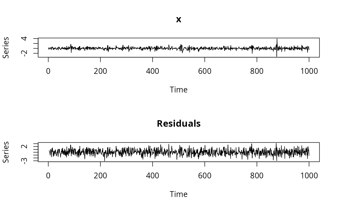
x <- ts(x[101:1100])
x.arch <- garch(x, order = c(0,2)) # Fit ARCH(2)
#>
#> ***** ESTIMATION WITH ANALYTICAL GRADIENT *****
#>
#>
#> I INITIAL X(I) D(I)
#>
#> 1 2.363190e-01 1.000e+00
#> 2 5.000000e-02 1.000e+00
#> 3 5.000000e-02 1.000e+00
#>
#> IT NF F RELDF PRELDF RELDX STPPAR D*STEP NPRELDF
#> 0 1 -2.325e+02
#> 1 3 -2.767e+02 1.60e-01 1.95e-01 1.7e-01 5.4e+03 1.0e-01 5.25e+02
#> 2 4 -2.960e+02 6.50e-02 8.53e-02 2.3e-01 2.8e+00 1.0e-01 2.47e+00
#> 3 5 -2.987e+02 8.98e-03 1.04e-01 1.7e-01 2.0e+00 1.0e-01 3.66e+02
#> 4 6 -3.149e+02 5.15e-02 4.21e-02 8.5e-02 2.0e+00 5.0e-02 6.29e+01
#> 5 8 -3.161e+02 3.78e-03 5.49e-03 2.6e-02 3.4e+00 1.9e-02 2.03e+01
#> 6 9 -3.175e+02 4.50e-03 5.92e-03 2.6e-02 2.0e+00 1.9e-02 1.43e+01
#> 7 10 -3.199e+02 7.52e-03 9.82e-03 5.3e-02 2.0e+00 3.9e-02 7.96e+00
#> 8 11 -3.222e+02 7.07e-03 1.54e-02 9.6e-02 2.0e+00 7.8e-02 2.03e+00
#> 9 13 -3.229e+02 2.14e-03 6.49e-03 2.7e-02 2.0e+00 3.6e-02 2.13e-01
#> 10 14 -3.237e+02 2.36e-03 3.49e-03 4.0e-02 2.0e+00 3.6e-02 1.75e-01
#> 11 15 -3.239e+02 7.96e-04 1.20e-03 3.0e-02 1.9e+00 3.6e-02 3.78e-02
#> 12 17 -3.240e+02 2.36e-04 4.66e-04 8.1e-03 7.1e+00 1.0e-02 4.45e-02
#> 13 18 -3.241e+02 2.92e-04 6.62e-04 7.8e-03 2.0e+00 1.0e-02 1.02e-01
#> 14 19 -3.242e+02 2.59e-04 4.09e-04 8.6e-03 2.0e+00 1.0e-02 1.73e-02
#> 15 20 -3.242e+02 2.77e-05 1.40e-04 8.7e-03 1.8e+00 1.0e-02 1.57e-03
#> 16 21 -3.242e+02 1.08e-04 1.23e-04 7.6e-03 8.3e-01 1.0e-02 1.67e-04
#> 17 23 -3.242e+02 6.68e-06 2.42e-05 2.8e-03 1.5e+00 3.0e-03 3.36e-05
#> 18 24 -3.242e+02 1.02e-05 1.27e-05 2.9e-03 5.7e-01 3.0e-03 1.40e-05
#> 19 25 -3.242e+02 8.70e-07 1.36e-06 1.1e-03 0.0e+00 1.2e-03 1.36e-06
#> 20 26 -3.242e+02 1.33e-07 1.34e-07 3.3e-04 0.0e+00 3.5e-04 1.34e-07
#> 21 27 -3.242e+02 1.50e-12 1.51e-12 9.0e-07 0.0e+00 1.0e-06 1.51e-12
#>
#> ***** RELATIVE FUNCTION CONVERGENCE *****
#>
#> FUNCTION -3.242267e+02 RELDX 8.952e-07
#> FUNC. EVALS 27 GRAD. EVALS 22
#> PRELDF 1.509e-12 NPRELDF 1.509e-12
#>
#> I FINAL X(I) D(I) G(I)
#>
#> 1 9.157780e-02 1.000e+00 1.712e-05
#> 2 5.183412e-01 1.000e+00 1.519e-06
#> 3 1.342126e-01 1.000e+00 9.057e-06
#>
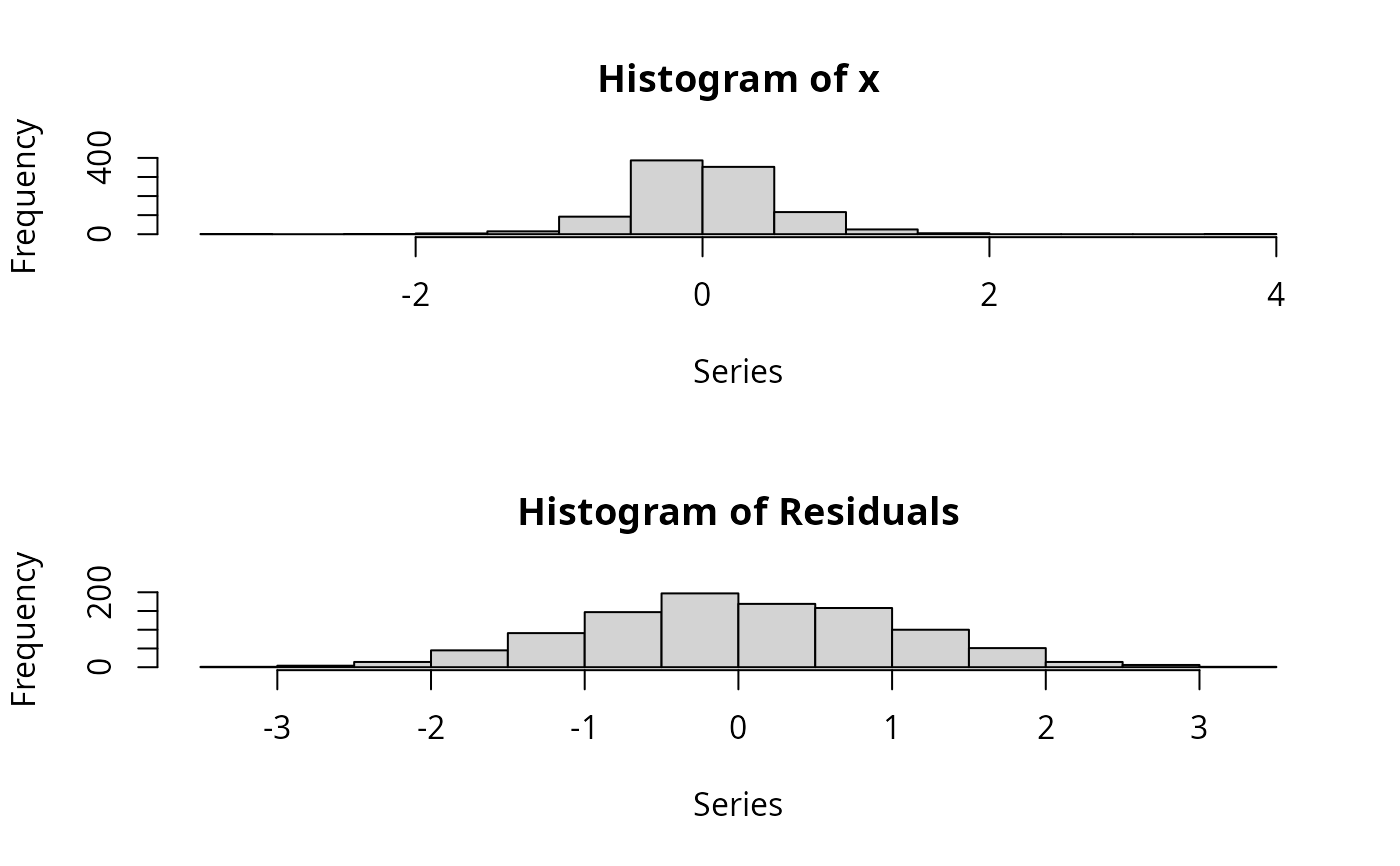
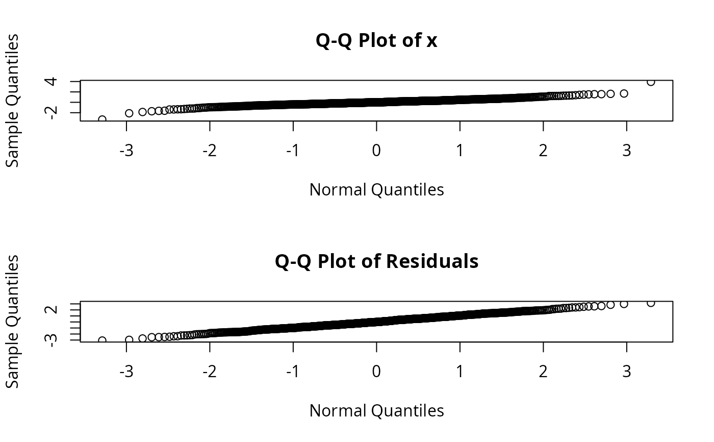
summary(x.arch) # Diagnostic tests
#>
#> Call:
#> garch(x = x, order = c(0, 2))
#>
#> Model:
#> GARCH(0,2)
#>
#> Residuals:
#> Min 1Q Median 3Q Max
#> -3.0820433 -0.6446973 -0.0002197 0.7076624 3.1693239
#>
#> Coefficient(s):
#> Estimate Std. Error t value Pr(>|t|)
#> a0 0.091578 0.008291 11.045 < 2e-16 ***
#> a1 0.518341 0.069238 7.486 7.08e-14 ***
#> a2 0.134213 0.045741 2.934 0.00334 **
#> ---
#> Signif. codes: 0 ‘***’ 0.001 ‘**’ 0.01 ‘*’ 0.05 ‘.’ 0.1 ‘ ’ 1
#>
#> Diagnostic Tests:
#> Jarque Bera Test
#>
#> data: Residuals
#> X-squared = 1.1825, df = 2, p-value = 0.5536
#>
#>
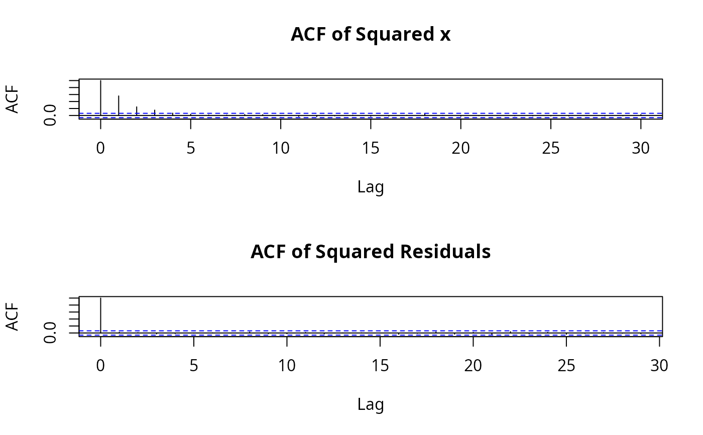
#> Box-Ljung test
#>
#> data: Squared.Residuals
#> X-squared = 0.3441, df = 1, p-value = 0.5575
#>
plot(x.arch)
 data(EuStockMarkets)
dax <- diff(log(EuStockMarkets))[,"DAX"]
dax.garch <- garch(dax) # Fit a GARCH(1,1) to DAX returns
#>
#> ***** ESTIMATION WITH ANALYTICAL GRADIENT *****
#>
#>
#> I INITIAL X(I) D(I)
#>
#> 1 9.549651e-05 1.000e+00
#> 2 5.000000e-02 1.000e+00
#> 3 5.000000e-02 1.000e+00
#>
#> IT NF F RELDF PRELDF RELDX STPPAR D*STEP NPRELDF
#> 0 1 -7.584e+03
#> 1 8 -7.585e+03 1.45e-05 2.60e-05 1.4e-05 1.0e+11 1.4e-06 1.35e+06
#> 2 9 -7.585e+03 1.88e-07 1.97e-07 1.3e-05 2.0e+00 1.4e-06 1.50e+00
#> 3 18 -7.589e+03 6.22e-04 1.10e-03 3.5e-01 2.0e+00 5.5e-02 1.50e+00
#> 4 21 -7.601e+03 1.58e-03 1.81e-03 6.2e-01 1.9e+00 2.2e-01 3.07e-01
#> 5 23 -7.634e+03 4.22e-03 3.55e-03 4.3e-01 9.6e-01 4.4e-01 3.06e-02
#> 6 25 -7.646e+03 1.61e-03 1.85e-03 2.9e-02 2.0e+00 4.4e-02 5.43e-02
#> 7 27 -7.646e+03 3.82e-05 5.23e-04 1.3e-02 2.0e+00 2.0e-02 1.46e-02
#> 8 28 -7.648e+03 1.86e-04 1.46e-04 6.5e-03 2.0e+00 9.9e-03 1.54e-03
#> 9 29 -7.648e+03 3.12e-05 4.83e-05 6.4e-03 2.0e+00 9.9e-03 3.34e-03
#> 10 30 -7.648e+03 1.39e-05 6.31e-05 6.2e-03 1.9e+00 9.9e-03 1.86e-03
#> 11 31 -7.650e+03 2.70e-04 3.24e-04 6.0e-03 1.9e+00 9.9e-03 4.99e-03
#> 12 34 -7.656e+03 8.42e-04 8.57e-04 2.2e-02 1.7e-01 3.9e-02 2.22e-03
#> 13 36 -7.661e+03 6.12e-04 6.40e-04 1.9e-02 4.2e-01 3.9e-02 2.09e-03
#> 14 38 -7.665e+03 4.87e-04 8.63e-04 4.9e-02 4.1e-01 9.6e-02 9.69e-04
#> 15 48 -7.666e+03 1.02e-04 1.86e-04 1.9e-07 4.5e+00 3.5e-07 3.94e-04
#> 16 49 -7.666e+03 1.12e-07 1.01e-07 1.9e-07 2.0e+00 3.5e-07 6.22e-05
#> 17 57 -7.666e+03 1.60e-05 2.70e-05 2.0e-03 9.3e-01 3.7e-03 6.10e-05
#> 18 59 -7.666e+03 5.23e-06 7.01e-06 3.7e-03 3.9e-01 8.0e-03 7.77e-06
#> 19 60 -7.666e+03 4.08e-08 3.74e-08 1.4e-04 0.0e+00 3.1e-04 3.74e-08
#> 20 61 -7.666e+03 2.31e-09 8.57e-10 8.6e-06 0.0e+00 2.0e-05 8.57e-10
#> 21 62 -7.666e+03 5.35e-11 2.25e-13 7.6e-07 0.0e+00 1.6e-06 2.25e-13
#> 22 63 -7.666e+03 1.81e-12 7.06e-16 1.7e-08 0.0e+00 3.4e-08 7.06e-16
#> 23 64 -7.666e+03 7.00e-14 1.69e-17 1.0e-09 0.0e+00 2.4e-09 1.69e-17
#> 24 65 -7.666e+03 -1.16e-14 1.76e-20 1.9e-10 0.0e+00 4.0e-10 1.76e-20
#>
#> ***** X- AND RELATIVE FUNCTION CONVERGENCE *****
#>
#> FUNCTION -7.665775e+03 RELDX 1.874e-10
#> FUNC. EVALS 65 GRAD. EVALS 24
#> PRELDF 1.760e-20 NPRELDF 1.760e-20
#>
#> I FINAL X(I) D(I) G(I)
#>
#> 1 4.639289e-06 1.000e+00 -2.337e-02
#> 2 6.832875e-02 1.000e+00 -8.294e-07
#> 3 8.890666e-01 1.000e+00 -2.230e-06
#>
summary(dax.garch) # ARCH effects are filtered. However,
#>
#> Call:
#> garch(x = dax)
#>
#> Model:
#> GARCH(1,1)
#>
#> Residuals:
#> Min 1Q Median 3Q Max
#> -12.18398 -0.47968 0.04949 0.65746 4.48048
#>
#> Coefficient(s):
#> Estimate Std. Error t value Pr(>|t|)
#> a0 4.639e-06 7.560e-07 6.137 8.42e-10 ***
#> a1 6.833e-02 1.125e-02 6.073 1.25e-09 ***
#> b1 8.891e-01 1.652e-02 53.817 < 2e-16 ***
#> ---
#> Signif. codes: 0 ‘***’ 0.001 ‘**’ 0.01 ‘*’ 0.05 ‘.’ 0.1 ‘ ’ 1
#>
#> Diagnostic Tests:
#> Jarque Bera Test
#>
#> data: Residuals
#> X-squared = 12947, df = 2, p-value < 2.2e-16
#>
#>
#> Box-Ljung test
#>
#> data: Squared.Residuals
#> X-squared = 0.13566, df = 1, p-value = 0.7126
#>
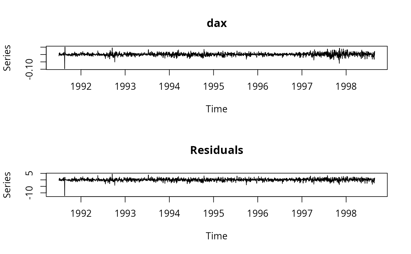
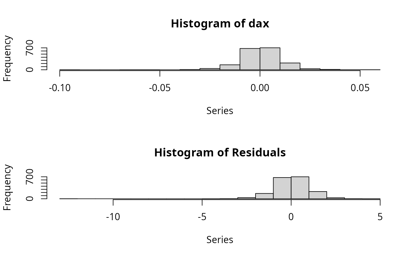
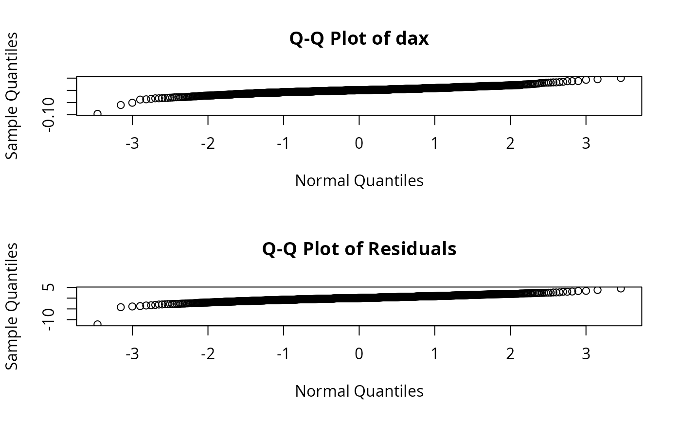
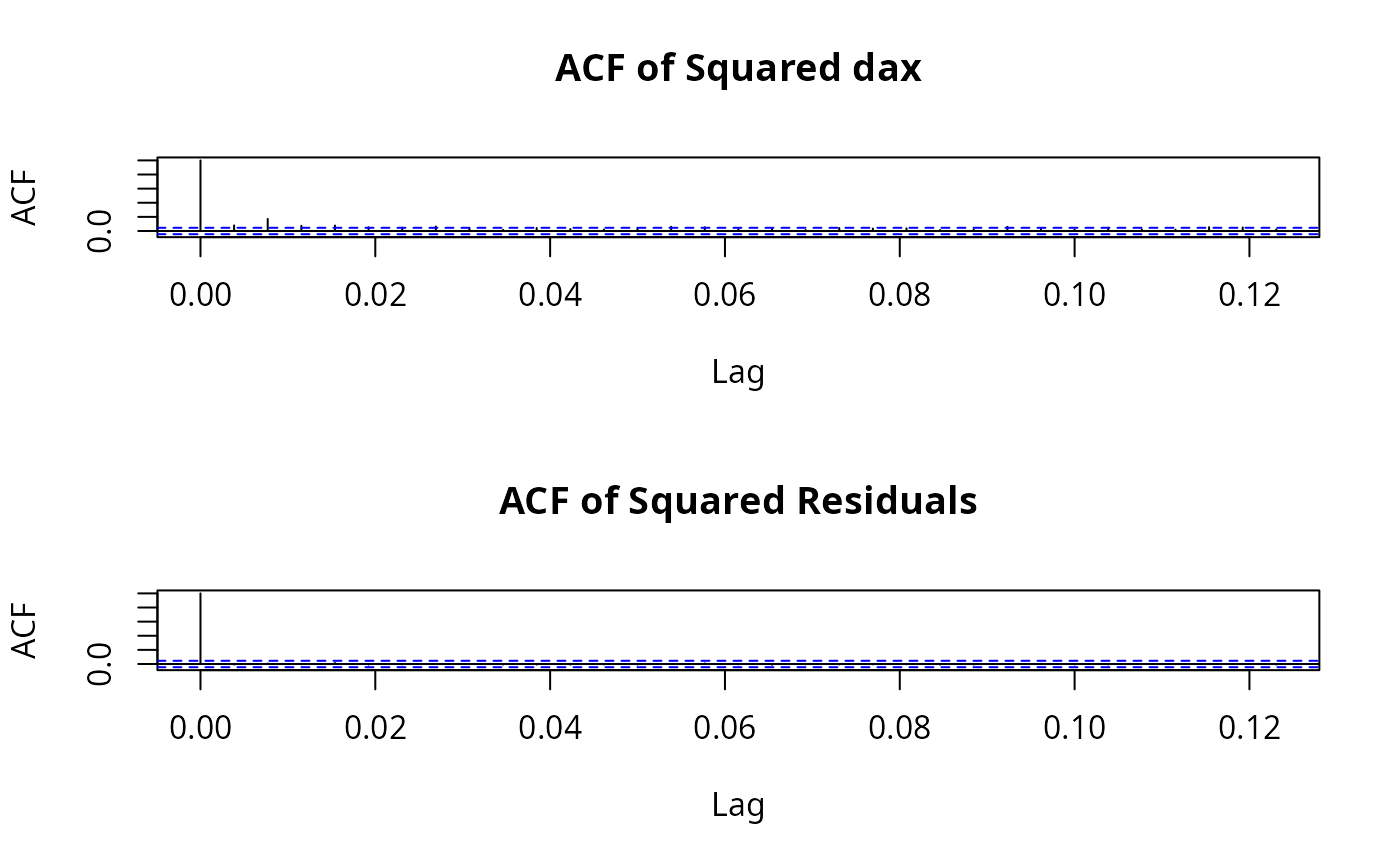
plot(dax.garch) # conditional normality seems to be violated
data(EuStockMarkets)
dax <- diff(log(EuStockMarkets))[,"DAX"]
dax.garch <- garch(dax) # Fit a GARCH(1,1) to DAX returns
#>
#> ***** ESTIMATION WITH ANALYTICAL GRADIENT *****
#>
#>
#> I INITIAL X(I) D(I)
#>
#> 1 9.549651e-05 1.000e+00
#> 2 5.000000e-02 1.000e+00
#> 3 5.000000e-02 1.000e+00
#>
#> IT NF F RELDF PRELDF RELDX STPPAR D*STEP NPRELDF
#> 0 1 -7.584e+03
#> 1 8 -7.585e+03 1.45e-05 2.60e-05 1.4e-05 1.0e+11 1.4e-06 1.35e+06
#> 2 9 -7.585e+03 1.88e-07 1.97e-07 1.3e-05 2.0e+00 1.4e-06 1.50e+00
#> 3 18 -7.589e+03 6.22e-04 1.10e-03 3.5e-01 2.0e+00 5.5e-02 1.50e+00
#> 4 21 -7.601e+03 1.58e-03 1.81e-03 6.2e-01 1.9e+00 2.2e-01 3.07e-01
#> 5 23 -7.634e+03 4.22e-03 3.55e-03 4.3e-01 9.6e-01 4.4e-01 3.06e-02
#> 6 25 -7.646e+03 1.61e-03 1.85e-03 2.9e-02 2.0e+00 4.4e-02 5.43e-02
#> 7 27 -7.646e+03 3.82e-05 5.23e-04 1.3e-02 2.0e+00 2.0e-02 1.46e-02
#> 8 28 -7.648e+03 1.86e-04 1.46e-04 6.5e-03 2.0e+00 9.9e-03 1.54e-03
#> 9 29 -7.648e+03 3.12e-05 4.83e-05 6.4e-03 2.0e+00 9.9e-03 3.34e-03
#> 10 30 -7.648e+03 1.39e-05 6.31e-05 6.2e-03 1.9e+00 9.9e-03 1.86e-03
#> 11 31 -7.650e+03 2.70e-04 3.24e-04 6.0e-03 1.9e+00 9.9e-03 4.99e-03
#> 12 34 -7.656e+03 8.42e-04 8.57e-04 2.2e-02 1.7e-01 3.9e-02 2.22e-03
#> 13 36 -7.661e+03 6.12e-04 6.40e-04 1.9e-02 4.2e-01 3.9e-02 2.09e-03
#> 14 38 -7.665e+03 4.87e-04 8.63e-04 4.9e-02 4.1e-01 9.6e-02 9.69e-04
#> 15 48 -7.666e+03 1.02e-04 1.86e-04 1.9e-07 4.5e+00 3.5e-07 3.94e-04
#> 16 49 -7.666e+03 1.12e-07 1.01e-07 1.9e-07 2.0e+00 3.5e-07 6.22e-05
#> 17 57 -7.666e+03 1.60e-05 2.70e-05 2.0e-03 9.3e-01 3.7e-03 6.10e-05
#> 18 59 -7.666e+03 5.23e-06 7.01e-06 3.7e-03 3.9e-01 8.0e-03 7.77e-06
#> 19 60 -7.666e+03 4.08e-08 3.74e-08 1.4e-04 0.0e+00 3.1e-04 3.74e-08
#> 20 61 -7.666e+03 2.31e-09 8.57e-10 8.6e-06 0.0e+00 2.0e-05 8.57e-10
#> 21 62 -7.666e+03 5.35e-11 2.25e-13 7.6e-07 0.0e+00 1.6e-06 2.25e-13
#> 22 63 -7.666e+03 1.81e-12 7.06e-16 1.7e-08 0.0e+00 3.4e-08 7.06e-16
#> 23 64 -7.666e+03 7.00e-14 1.69e-17 1.0e-09 0.0e+00 2.4e-09 1.69e-17
#> 24 65 -7.666e+03 -1.16e-14 1.76e-20 1.9e-10 0.0e+00 4.0e-10 1.76e-20
#>
#> ***** X- AND RELATIVE FUNCTION CONVERGENCE *****
#>
#> FUNCTION -7.665775e+03 RELDX 1.874e-10
#> FUNC. EVALS 65 GRAD. EVALS 24
#> PRELDF 1.760e-20 NPRELDF 1.760e-20
#>
#> I FINAL X(I) D(I) G(I)
#>
#> 1 4.639289e-06 1.000e+00 -2.337e-02
#> 2 6.832875e-02 1.000e+00 -8.294e-07
#> 3 8.890666e-01 1.000e+00 -2.230e-06
#>
summary(dax.garch) # ARCH effects are filtered. However,
#>
#> Call:
#> garch(x = dax)
#>
#> Model:
#> GARCH(1,1)
#>
#> Residuals:
#> Min 1Q Median 3Q Max
#> -12.18398 -0.47968 0.04949 0.65746 4.48048
#>
#> Coefficient(s):
#> Estimate Std. Error t value Pr(>|t|)
#> a0 4.639e-06 7.560e-07 6.137 8.42e-10 ***
#> a1 6.833e-02 1.125e-02 6.073 1.25e-09 ***
#> b1 8.891e-01 1.652e-02 53.817 < 2e-16 ***
#> ---
#> Signif. codes: 0 ‘***’ 0.001 ‘**’ 0.01 ‘*’ 0.05 ‘.’ 0.1 ‘ ’ 1
#>
#> Diagnostic Tests:
#> Jarque Bera Test
#>
#> data: Residuals
#> X-squared = 12947, df = 2, p-value < 2.2e-16
#>
#>
#> Box-Ljung test
#>
#> data: Squared.Residuals
#> X-squared = 0.13566, df = 1, p-value = 0.7126
#>
plot(dax.garch) # conditional normality seems to be violated