Smoothing splines using a pspline basis

Specifies a penalised spline basis for the predictor. This is done by fitting a comparatively small set of splines and penalising the integrated second derivative. Traditional smoothing splines use one basis per observation, but several authors have pointed out that the final results of the fit are indistinguishable for any number of basis functions greater than about 2-3 times the degrees of freedom. Eilers and Marx point out that if the basis functions are evenly spaced, this leads to significant computational simplification, they refer to the result as a p-spline.

Usage

pspline(x, df=4, theta, nterm=2.5 * df, degree=3, eps=0.1, method,
   Boundary.knots=range(x), intercept=FALSE, penalty=TRUE, combine, ...)

psplineinverse(x)

Arguments

x: for psline: a covariate vector. The function does not apply to factor variables. For psplineinverse x will be the result of a pspline call.
df: the desired degrees of freedom. One of the arguments df or theta' must be given, but not both. If df=0, then the AIC = (loglik -df) is used to choose an "optimal" degrees of freedom. If AIC is chosen, then an optional argument `caic=T' can be used to specify the corrected AIC of Hurvich et. al.
theta: roughness penalty for the fit. It is a monotone function of the degrees of freedom, with theta=1 corresponding to a linear fit and theta=0 to an unconstrained fit of nterm degrees of freedom.
nterm: number of splines in the basis
degree: degree of splines
eps: accuracy for df
method: the method for choosing the tuning parameter theta. If theta is given, then 'fixed' is assumed. If the degrees of freedom is given, then 'df' is assumed. If method='aic' then the degrees of freedom is chosen automatically using Akaike's information criterion.
...: optional arguments to the control function
Boundary.knots: the spline is linear beyond the boundary knots. These default to the range of the data.
intercept: if TRUE, the basis functions include the intercept.
penalty: if FALSE a large number of attributes having to do with penalized fits are excluded. This is useful to create a pspline basis matrix for other uses.
combine: an optional vector of increasing integers. If two adjacent values of combine are equal, then the corresponding coefficients of the fit are forced to be equal. This is useful for monotone fits, see the vignette for more details.

Value

Object of class pspline, coxph.penalty containing the spline basis, with the appropriate attributes to be recognized as a penalized term by the coxph or survreg functions.

For psplineinverse the original x vector is reconstructed.

References

Eilers, Paul H. and Marx, Brian D. (1996). Flexible smoothing with B-splines and penalties. Statistical Science, 11, 89-121.

Hurvich, C.M. and Simonoff, J.S. and Tsai, Chih-Ling (1998). Smoothing parameter selection in nonparametric regression using an improved Akaike information criterion, JRSSB, volume 60, 271–293.

Examples

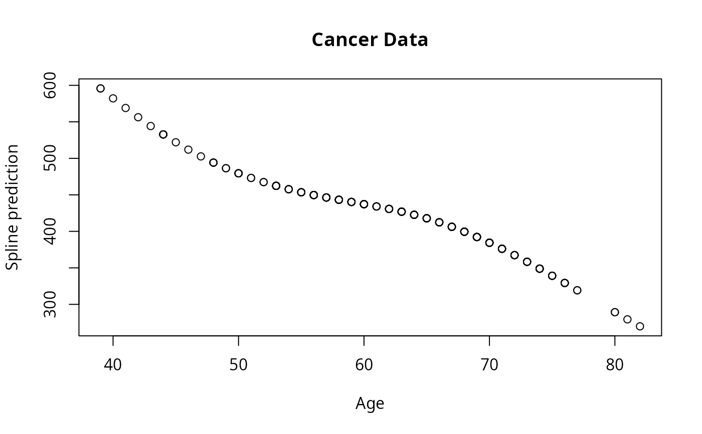
lfit6 <- survreg(Surv(time, status)~pspline(age, df=2), lung)
plot(lung$age, predict(lfit6), xlab='Age', ylab="Spline prediction")
title("Cancer Data")

fit0 <- coxph(Surv(time, status) ~ ph.ecog + age, lung)
fit1 <- coxph(Surv(time, status) ~ ph.ecog + pspline(age,3), lung)
fit3 <- coxph(Surv(time, status) ~ ph.ecog + pspline(age,8), lung)
fit0
#> Call:
#> coxph(formula = Surv(time, status) ~ ph.ecog + age, data = lung)
#> 
#>             coef exp(coef) se(coef)     z        p
#> ph.ecog 0.443485  1.558128 0.115831 3.829 0.000129
#> age     0.011281  1.011345 0.009319 1.211 0.226082
#> 
#> Likelihood ratio test=19.06  on 2 df, p=7.279e-05
#> n= 227, number of events= 164 
#>    (1 observation deleted due to missingness)
fit1
#> Call:
#> coxph(formula = Surv(time, status) ~ ph.ecog + pspline(age, 3), 
#>     data = lung)
#> 
#>                             coef se(coef)      se2    Chisq   DF       p
#> ph.ecog                  0.44802  0.11707  0.11678 14.64453 1.00 0.00013
#> pspline(age, 3), linear  0.01126  0.00928  0.00928  1.47231 1.00 0.22498
#> pspline(age, 3), nonlin                             2.07924 2.08 0.37143
#> 
#> Iterations: 4 outer, 12 Newton-Raphson
#>      Theta= 0.861 
#> Degrees of freedom for terms= 1.0 3.1 
#> Likelihood ratio test=21.9  on 4.08 df, p=2e-04
#> n= 227, number of events= 164 
#>    (1 observation deleted due to missingness)
fit3
#> Call:
#> coxph(formula = Surv(time, status) ~ ph.ecog + pspline(age, 8), 
#>     data = lung)
#> 
#>                             coef se(coef)      se2    Chisq   DF       p
#> ph.ecog                  0.47640  0.12024  0.11925 15.69732 1.00 7.4e-05
#> pspline(age, 8), linear  0.01172  0.00923  0.00923  1.61161 1.00    0.20
#> pspline(age, 8), nonlin                             6.93188 6.99    0.43
#> 
#> Iterations: 5 outer, 15 Newton-Raphson
#>      Theta= 0.691 
#> Degrees of freedom for terms= 1 8 
#> Likelihood ratio test=27.6  on 8.97 df, p=0.001
#> n= 227, number of events= 164 
#>    (1 observation deleted due to missingness)