Add Lines or Points to a Survival Plot

Often used to add the expected survival curve(s) to a Kaplan-Meier plot generated with plot.survfit.

Usage

# S3 method for class 'survfit'
lines(x, type="s", pch=3, col=1, lty=1,
        lwd=1, cex=1, mark.time=FALSE, xmax,
        fun, conf.int=FALSE,
        conf.times, conf.cap=.005, conf.offset=.012,
        conf.type = c("log", "log-log", "plain", "logit", "arcsin"),
        mark, noplot="(s0)", cumhaz= FALSE,  cumprob= FALSE, ...)
# S3 method for class 'survexp'
lines(x, type="l", ...)
# S3 method for class 'survfit'
points(x, fun, censor=FALSE, col=1, pch,
        noplot="(s0)", cumhaz=FALSE, ...)

Arguments

x: a survival object, generated from the survfit or survexp functions.
type: the line type, as described in lines. The default is a step function for survfit objects, and a connected line for survexp objects. All other arguments for lines.survexp are identical to those for lines.survfit.
col, lty, lwd, cex: vectors giving the mark symbol, color, line type, line width and character size for the added curves. Of this set only color is applicable to points.
pch: plotting characters for points, in the style of matplot, i.e., either a single string of characters of which the first will be used for the first curve, etc; or a vector of characters or integers, one element per curve.
mark: a historical alias for pch
censor: should censoring times be displayed for the points function?
mark.time: controls the labeling of the curves. If FALSE, no labeling is done. If TRUE, then curves are marked at each censoring time. If mark.time is a numeric vector, then curves are marked at the specified time points.
xmax: optional cutoff for the right hand of the curves.
fun: an arbitrary function defining a transformation of the survival curve. For example fun=log is an alternative way to draw a log-survival curve (but with the axis labeled with log(S) values). Four often used transformations can be specified with a character argument instead: "log" is the same as using the log=T option, "event" plots cumulative events (f(y) = 1-y), "cumhaz" plots the cumulative hazard function (f(y) = -log(y)) and "cloglog" creates a complimentary log-log survival plot (f(y) = log(-log(y))) along with log scale for the x-axis.
conf.int: if TRUE, confidence bands for the curves are also plotted. If set to "only", then only the CI bands are plotted, and the curve itself is left off. This can be useful for fine control over the colors or line types of a plot.
conf.times: optional vector of times at which to place a confidence bar on the curve(s). If present, these will be used instead of confidence bands.
conf.cap: width of the horizontal cap on top of the confidence bars; only used if conf.times is used. A value of 1 is the width of the plot region.
conf.offset: the offset for confidence bars, when there are multiple curves on the plot. A value of 1 is the width of the plot region. If this is a single number then each curve's bars are offset by this amount from the prior curve's bars, if it is a vector the values are used directly.
conf.type: One of "plain", "log" (the default), "log-log", "logit", or "none". Only enough of the string to uniquely identify it is necessary. The first option causes confidence intervals not to be generated. The second causes the standard intervals curve +- k *se(curve), where k is determined from conf.int. The log option calculates intervals based on the cumulative hazard or log(survival). The log-log option bases the intervals on the log hazard or log(-log(survival)), and the logit option on log(survival/(1-survival)).
noplot: for multi-state models, curves with this label will not be plotted. The default corresponds to an unspecified state.
cumhaz: plot the cumulative hazard, rather than the survival or probability in state.
cumprob: for a multi-state curve, plot the probabilities in state 1, (state1 + state2), (state1 + state2 + state3), .... If cumprob is an integer vector the totals will be in the order indicated.
...: other graphical parameters

Value

a list with components x and y, containing the coordinates of the last point on each of the curves (but not of the confidence limits). This may be useful for labeling. If cumprob=TRUE then y will be a matrix with one row per curve and x will be all the time points. This may be useful for adding shading.

Side Effects

one or more curves are added to the current plot.

Details

When the survfit function creates a multi-state survival curve the resulting object has class `survfitms'. The only difference in the plots is that that it defaults to a curve that goes from lower left to upper right (starting at 0), where survival curves default to starting at 1 and going down. All other options are identical.

If the user set an explicit range in an earlier plot.survfit call, e.g. via xlim or xmax, subsequent calls to this function remember the right hand cutoff. This memory can be erased by options(plot.survfit) <- NULL.

Examples

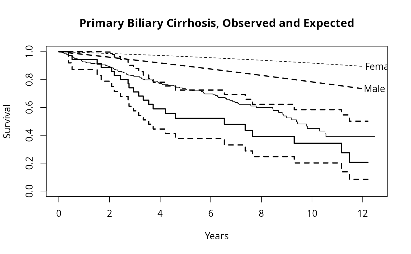
fit <- survfit(Surv(time, status==2) ~ sex, pbc,subset=1:312)
plot(fit, mark.time=FALSE, xscale=365.25,
        xlab='Years', ylab='Survival')
lines(fit[1], lwd=2)    #darken the first curve and add marks


# Add expected survival curves for the two groups,
#   based on the US census data
# The data set does not have entry date, use the midpoint of the study
efit <- survexp(~sex, data=pbc, times= (0:24)*182, ratetable=survexp.us, 
                 rmap=list(sex=sex, age=age*365.35, year=as.Date('1979/01/01')))
temp <- lines(efit, lty=2, lwd=2:1)
text(temp, c("Male", "Female"), adj= -.1) #labels just past the ends
title(main="Primary Biliary Cirrhosis, Observed and Expected")