Estimate survival function.

Estimates the survival function using a weighted Kaplan-Meier estimator.

Usage

svykm(formula, design,se=FALSE, ...)
# S3 method for class 'svykm'
plot(x,xlab="time",ylab="Proportion surviving",
  ylim=c(0,1),ci=NULL,lty=1,...)
# S3 method for class 'svykm'
lines(x,xlab="time",type="s",ci=FALSE,lty=1,...)
# S3 method for class 'svykmlist'
plot(x, pars=NULL, ci=FALSE,...)
# S3 method for class 'svykm'
quantile(x, probs=c(0.75,0.5,0.25),ci=FALSE,level=0.95,...)
# S3 method for class 'svykm'
confint(object,parm,level=0.95,...)

Arguments

formula: Two-sided formula. The response variable should be a right-censored Surv object
design: survey design object
se: Compute standard errors? This is slow for moderate to large data sets
...: in plot and lines methods, graphical parameters
x: a svykm or svykmlist object
xlab,ylab,ylim,type: as for plot
lty: Line type, see par
ci: Plot (or return, forquantile) the confidence interval
pars: A list of vectors of graphical parameters for the separate curves in a svykmlist object
object: A svykm object
parm: vector of times to report confidence intervals
level: confidence level
probs: survival probabilities for computing survival quantiles (note that these are the complement of the usual quantile input, so 0.9 means 90% surviving, not 90% dead)

Value

For svykm, an object of class svykm for a single curve or svykmlist for multiple curves.

Details

When standard errors are computed, the survival curve is actually the Aalen (hazard-based) estimator rather than the Kaplan-Meier estimator.

The standard error computations use memory proportional to the sample size times the square of the number of events. This can be a lot.

In the case of equal-probability cluster sampling without replacement the computations are essentially the same as those of Williams (1995), and the same linearization strategy is used for other designs.

Confidence intervals are computed on the log(survival) scale, following the default in survival package, which was based on simulations by Link(1984).

Confidence intervals for quantiles use Woodruff's method: the interval is the intersection of the horizontal line at the specified quantile with the pointwise confidence band around the survival curve.

References

Link, C. L. (1984). Confidence intervals for the survival function using Cox's proportional hazards model with covariates. Biometrics 40, 601-610.

Williams RL (1995) "Product-Limit Survival Functions with Correlated Survival Times" Lifetime Data Analysis 1: 171–186

Woodruff RS (1952) Confidence intervals for medians and other position measures. JASA 57, 622-627.

Examples

data(pbc, package="survival")
pbc$randomized <- with(pbc, !is.na(trt) & trt>0)
biasmodel<-glm(randomized~age*edema,data=pbc)
pbc$randprob<-fitted(biasmodel)

dpbc<-svydesign(id=~1, prob=~randprob, strata=~edema, data=subset(pbc,randomized))

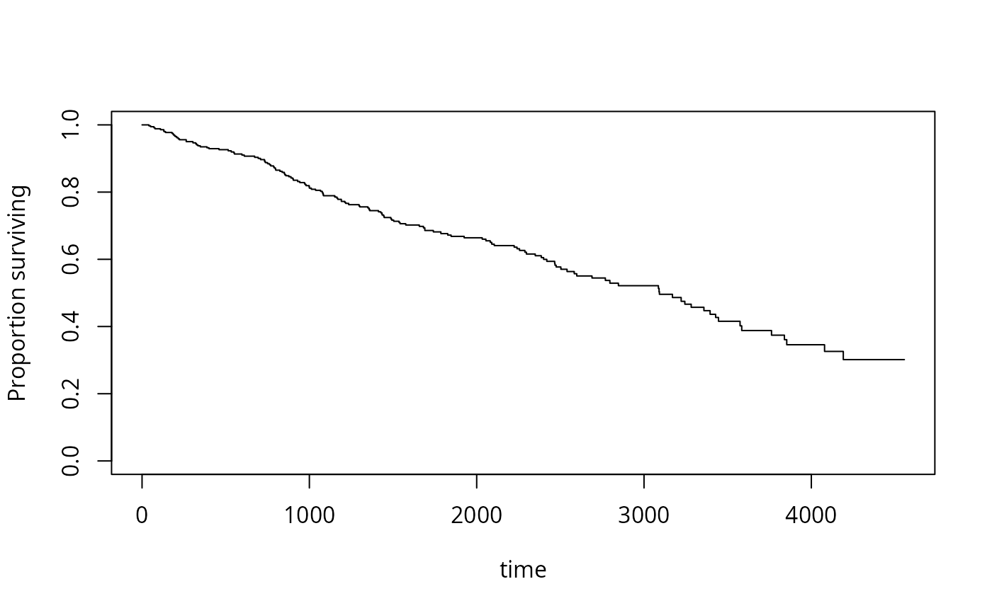
s1<-svykm(Surv(time,status>0)~1, design=dpbc)
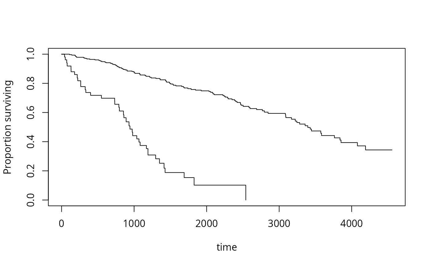
s2<-svykm(Surv(time,status>0)~I(bili>6), design=dpbc)

plot(s1)

plot(s2)

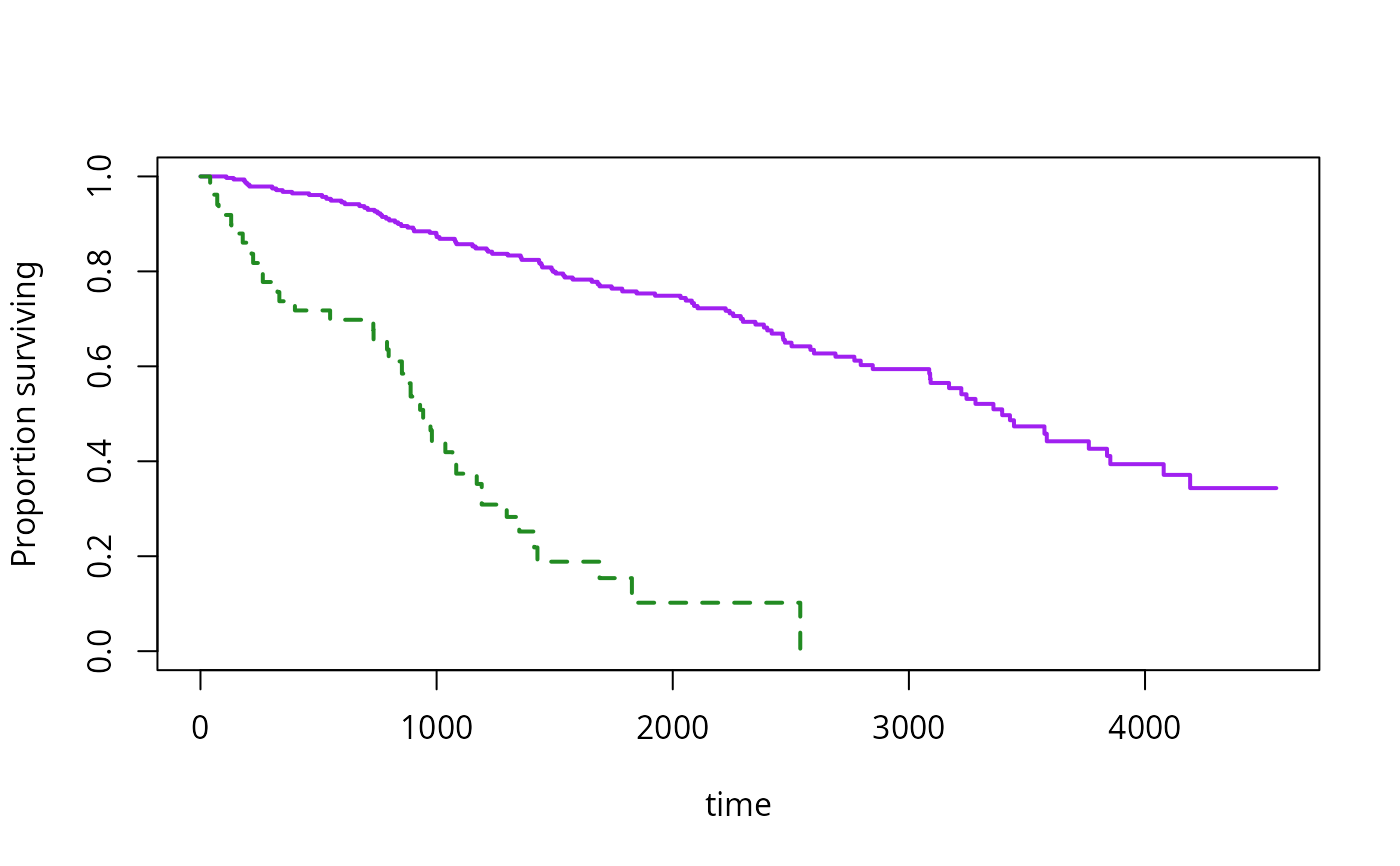
plot(s2, lwd=2, pars=list(lty=c(1,2),col=c("purple","forestgreen")))


quantile(s1, probs=c(0.9,0.75,0.5,0.25,0.1))
#>  0.9 0.75  0.5 0.25  0.1 
#>  708 1356 3092  Inf  Inf 

s3<-svykm(Surv(time,status>0)~I(bili>6), design=dpbc,se=TRUE)
plot(s3[[2]],col="purple")


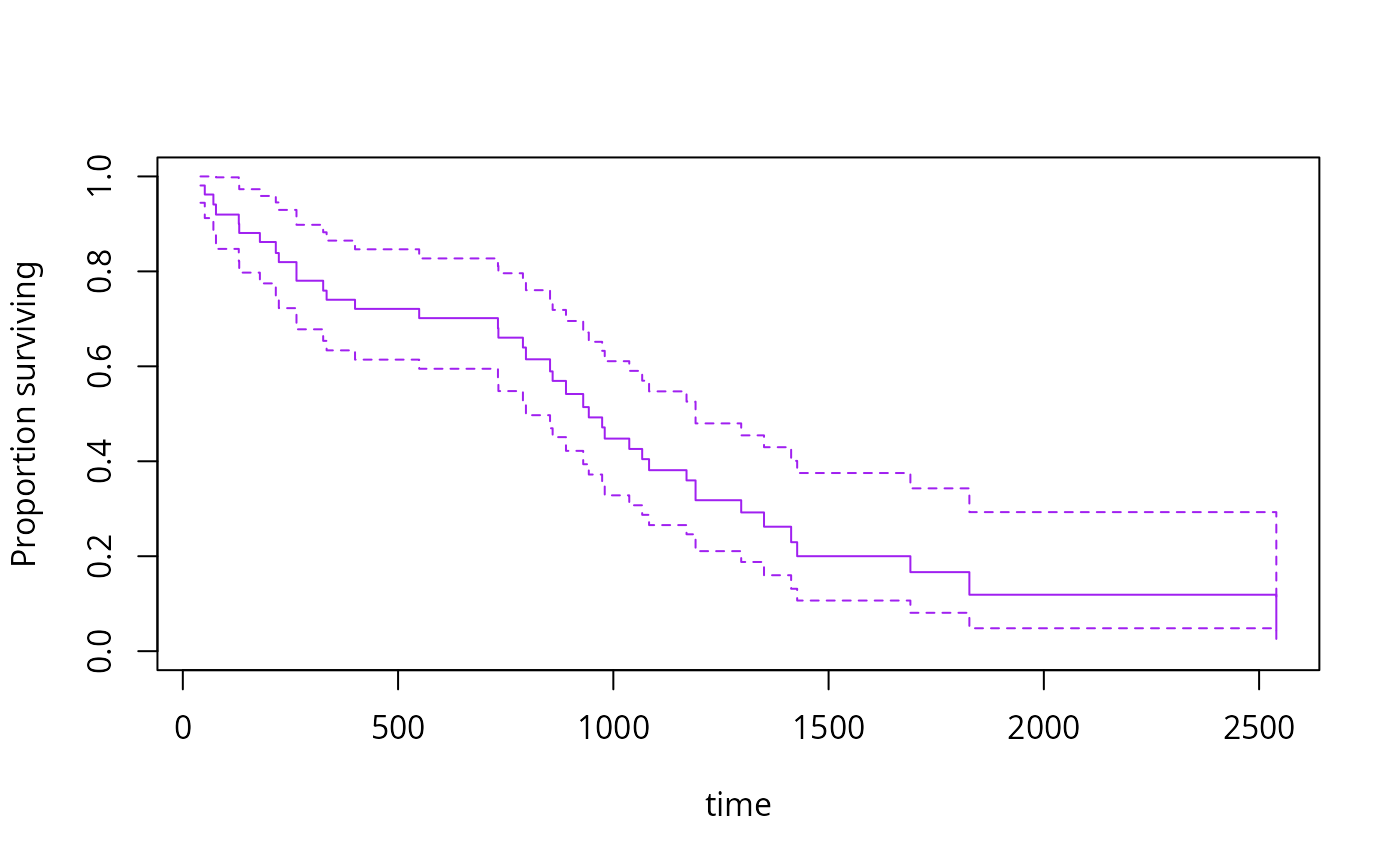confint(s3[[2]], parm=365*(1:5))
#>           0.025     0.975
#> 365  0.63361572 0.8647973
#> 730  0.59486017 0.8272783
#> 1095 0.26557946 0.5472405
#> 1460 0.10663428 0.3752484
#> 1825 0.08082427 0.3429355
quantile(s3[[1]], ci=TRUE)
#> 0.75  0.5 0.25 
#> 1925 3395  Inf 
#> attr(,"ci")
#>      0.025 0.975
#> 0.75  1504  2386
#> 0.5   3092  4079
#> 0.25   Inf   Inf