Reweight (optimise) the weights on frames

Evaluates a set of expressions for different frame weights in a dual-frame/multi-frame design, so that an optimal or compromise-optimal set of frame weights can be chosen

Usage

reweight(design, ...)
# S3 method for class 'dualframe'
reweight(design, targets=NULL, totals=NULL,
                             estimator=c("constant","expected"),
                             theta=NULL, theta_grid=seq(0,1,by=0.05),...)
# S3 method for class 'dualframe_with_rewt'
plot(x,y,type="b",...)

Arguments

design: dual-frame or multiframe design object
targets, totals: A list of quoted expressions estimating the variance of a survey estimator (targets), or a list of formulas that will be turned into targets for the variances of totals.
estimator: As in multiframe: "constant" is a constant weight for all observations in an overlap between frames, "expected" weights by the reciprocal of the expected numbers of times a unit is sampled and is not optimisable.
theta: As in multiframe, a fixed weight for observations in frame 1 also sampled in frame 2
theta_grid: Grid for optimising theta over, with estimator="constant"
x: object produced by reweight
y: ignored
type,...: in the plot method these are passed to matplot

Details

Traditionally, this optimisation has been done with totals, which is a good default and more mathematically tractable. However, when the point of multiple-frame sampling is to improve precision for a rare sub-population, or when you're doing regression modelling, you might want to optimise for something else.

Value

An object of class "dualframe_with_rewt".

The coef method returns the optimal theta for each target. The rewt element includes the variances of each target on a grid of theta in variances

Examples

data(phoneframes)
A_in_frames<-cbind(1, DatA$Domain=="ab")
B_in_frames<-cbind(DatB$Domain=="ba",1)

Bdes_pps<-svydesign(id=~1, fpc=~ProbB, data=DatB,pps=ppsmat(PiklB))
Ades_pps <-svydesign(id=~1, fpc=~ProbA,data=DatA,pps=ppsmat(PiklA))

## Not very good weighting
mf_pps<-multiframe(list(Ades_pps,Bdes_pps),list(A_in_frames,B_in_frames),theta=0.5) 
svytotal(~Lei+Feed+Tax+Clo,mf_pps, na.rm=TRUE)
#>       total      SE
#> Lei   52082  1458.9
#> Feed 575470 18075.2
#> Tax  205157  7231.1
#> Clo   70450  2395.1

## try to optimise
mf_opt<-reweight(mf_pps, totals=list(~Lei, ~Feed,~Tax,~Clo))
coef(mf_opt)
#> [1] 0.75 0.80 0.90 0.75
plot(mf_opt)


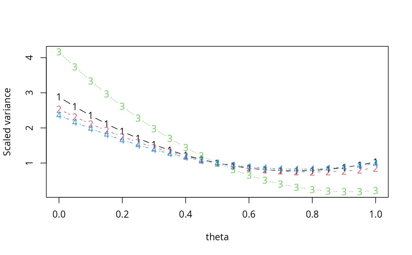## a good compromise is 0.80 for everything except Tax
## and it's still pretty good there
## (Tax will be biased because it's missing for landline-only)
mf_pps_opt<-reweight(mf_opt,theta=0.80) 
svytotal(~Lei+Feed+Tax+Clo,mf_pps_opt, na.rm=TRUE)
#>       total      SE
#> Lei   53544  1296.2
#> Feed 586855 15613.8
#> Tax  212601  3574.0
#> Clo   72234  2181.7


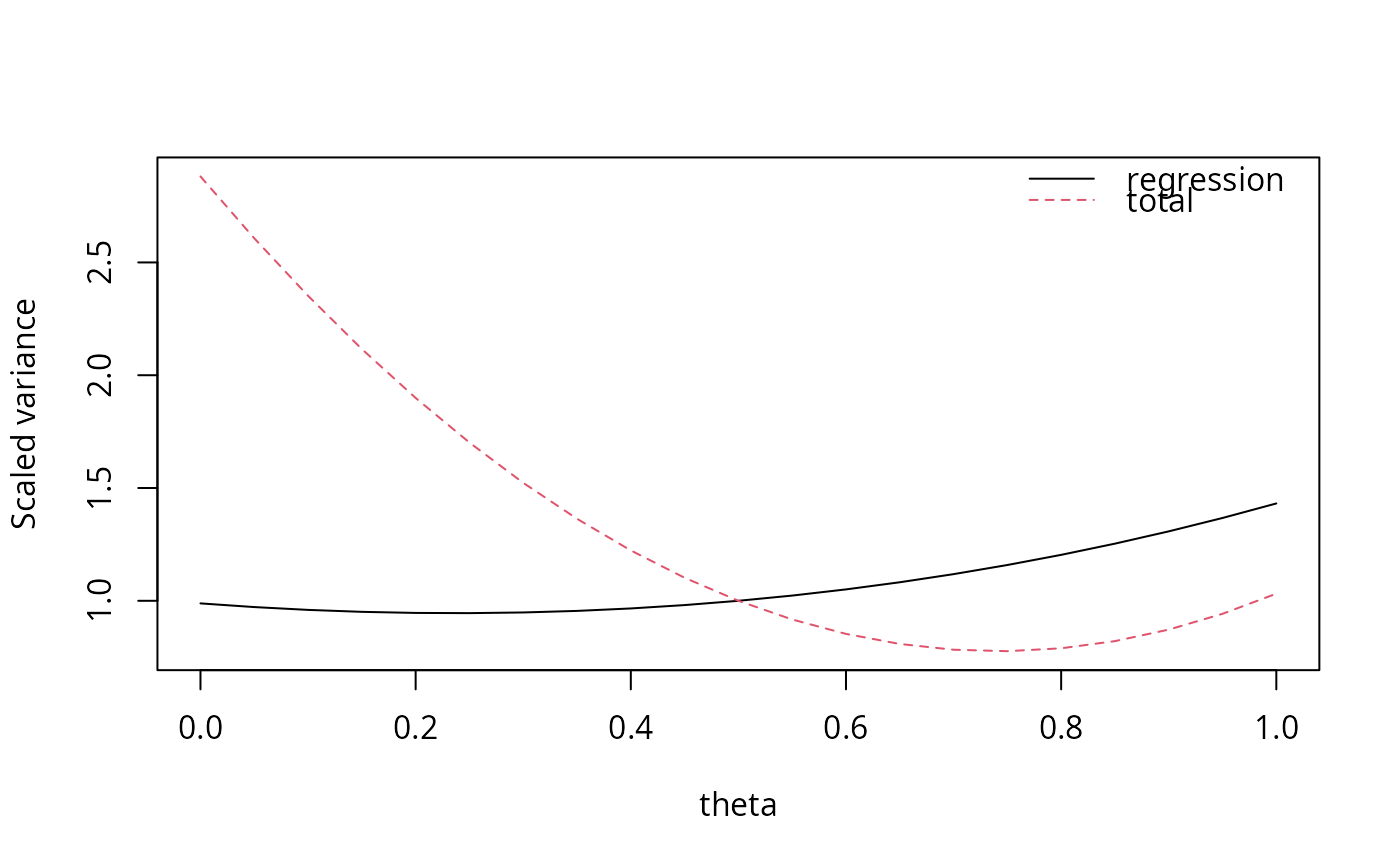
## Targets other than totals
mf_reg<-reweight(mf_pps,
  targets=list(quote(vcov(svyglm(Lei~Feed+Clo, design=.DESIGN))[1,1]),
               quote(vcov(svytotal(~Lei,.DESIGN))))
  )
plot(mf_reg,type="l")
legend("topright",bty="n",lty=1:2,col=1:2, legend=c("regression","total"))


## Zooming in on optimality for a particular variable (for compatibility)
mf_opt1<-reweight(mf_pps, totals=list(~Feed),theta_grid=seq(0.7,0.9,length=100))
coef(mf_opt1) # Frames2::Hartley gives 0.802776
#> [1] 0.8030303