Image or contour method for gridded spatial data; convert to and from image data structure

Create image for gridded data in SpatialGridDataFrame or SpatialPixelsDataFrame objects.

Usage

# S3 method for class 'SpatialGridDataFrame'
image(x, attr = 1, xcol = 1, ycol = 2, 
  col = heat.colors(12), red=NULL, green=NULL, blue=NULL,
        axes = FALSE, xlim = NULL,
  ylim = NULL, add = FALSE, ..., asp = NA, setParUsrBB=FALSE,
        interpolate = FALSE, angle = 0, 
  useRasterImage = !(.Platform$GUI[1] == "Rgui" &&
        getIdentification() == "R Console") && missing(breaks), breaks,
  zlim = range(as.numeric(x[[attr]])[is.finite(x[[attr]])]))
# S3 method for class 'SpatialPixelsDataFrame'
image(x, ...) 
# S3 method for class 'SpatialPixels'
image(x, ...) 
# S3 method for class 'SpatialGridDataFrame'
contour(x, attr = 1, xcol = 1, ycol = 2,
  col = 1, add = FALSE, xlim = NULL, ylim = NULL, axes = FALSE,
         ..., setParUsrBB = FALSE)
# S3 method for class 'SpatialPixelsDataFrame'
contour(x, ...) 
as.image.SpatialGridDataFrame(x, xcol = 1, ycol = 2, attr = 1)
image2Grid(im, p4 = as.character(NA), digits=10)

Arguments

x: object of class SpatialGridDataFrame
attr: column of attribute variable; this may be the column name in the data.frame of data (as.data.frame(data)), or a column number
xcol: column number of x-coordinate, in the coordinate matrix
ycol: column number of y-coordinate, in the coordinate matrix
col: a vector of colors
red,green,blue: columns names or numbers given instead of the attr argument when the data represent an image encoded in three colour bands on the 0-255 integer scale; all three columns must be given in this case, and the attribute values will be constructed using function rgb

axes: logical; should coordinate axes be drawn?
xlim: x-axis limits
ylim: y-axis limits
zlim: data limits for plotting the (raster, attribute) values
add: logical; if FALSE, the image is added to the plot layout setup by plot(as(x, "Spatial"),axes=axes,xlim=xlim,ylim=ylim,asp=asp) which sets up axes and plotting region; if TRUE, the image is added to the existing plot.
...: arguments passed to image, see examples
asp: aspect ratio to be used for plot
setParUsrBB: default FALSE, see Spatial-class for further details
useRasterImage: if TRUE, use rasterImage to render the image if available; for legacy rendering set FALSE; should be FALSE on Windows SDI installations
breaks: class breaks for coloured values
interpolate: default FALSE, a logical vector (or scalar) indicating whether to apply linear interpolation to the image when drawing, see rasterImage
angle: default 0, angle of rotation (in degrees, anti-clockwise from positive x-axis, about the bottom-left corner), see rasterImage
im: list with components named x, y, and z, as used for image
p4: CRS object, proj4 string
digits: default 10, number of significant digits to use for checking equal row/column spacing

Value

as.image.SpatialGridDataFrame returns the list with elements x and y, containing the coordinates of the cell centres of a matrix z, containing the attribute values in matrix form as needed by image.

Note

Providing xcol and ycol attributes seems obsolete, and it is for 2D data, but it may provide opportunities for plotting certain slices in 3D data. I haven't given this much thought yet.

filled.contour seems to misinterpret the coordinate values, if we take the image.default manual page as the reference.

Author

Edzer Pebesma

Examples

data(meuse.grid)
coordinates(meuse.grid) = c("x", "y") # promote to SpatialPointsDataFrame
gridded(meuse.grid) = TRUE            # promote to SpatialGridDataFrame
data(meuse)
coordinates(meuse) = c("x", "y")
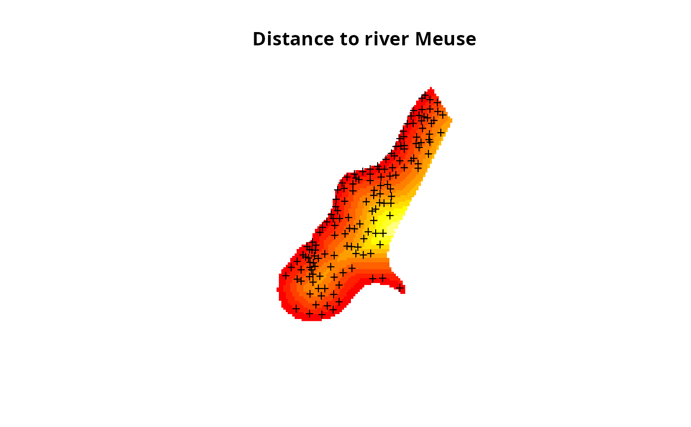
image(meuse.grid["dist"], main = "Distance to river Meuse")
points(coordinates(meuse), pch = "+")

image(meuse.grid["dist"], main = "Distance to river Meuse",
 useRasterImage=TRUE)
points(coordinates(meuse), pch = "+")


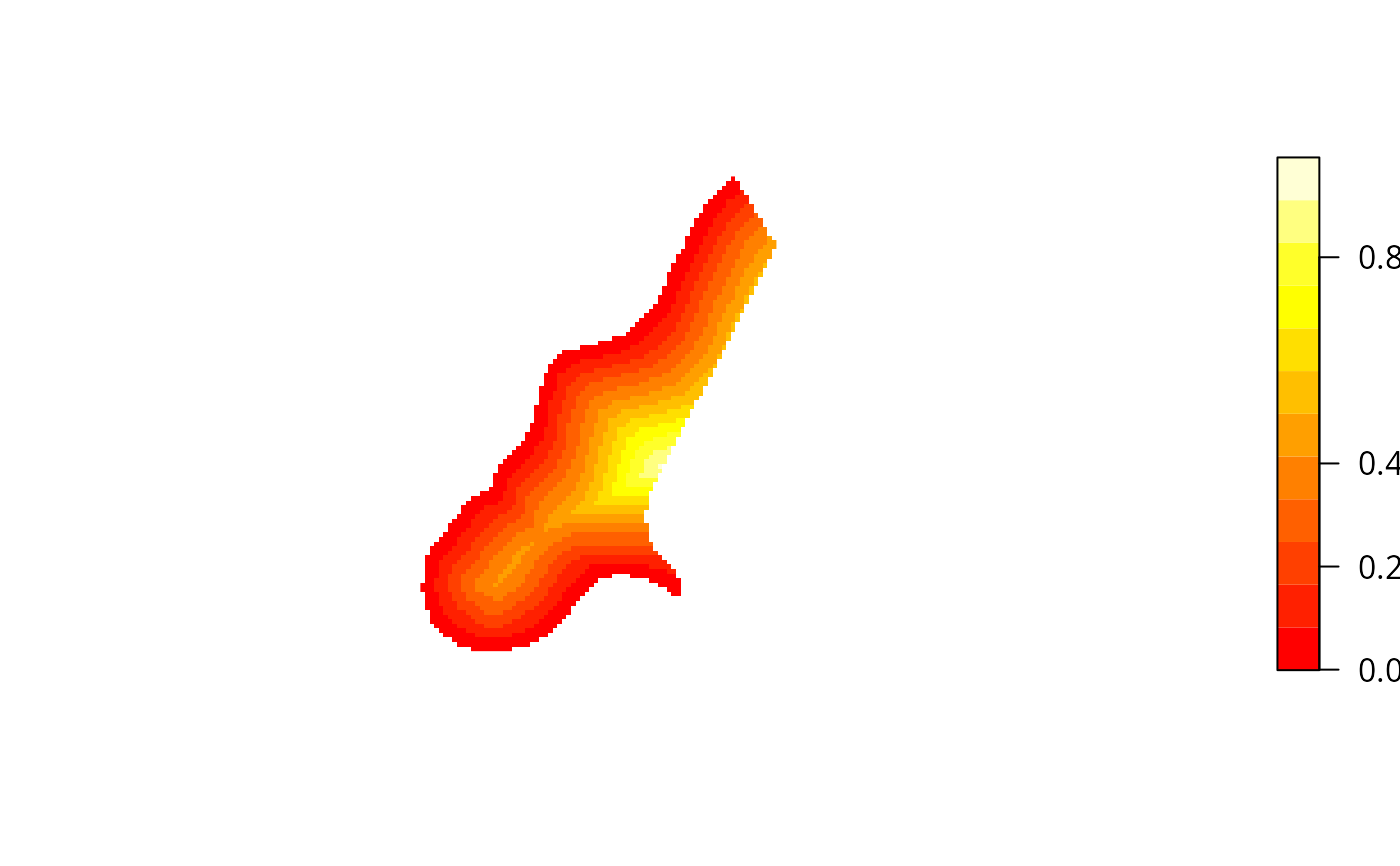
# color scale:
layout(cbind(1,2), c(4,1),1)
image(meuse.grid["dist"])
imageScale(meuse.grid$dist, axis.pos=4, add.axis=FALSE)
axis(4,at=c(0,.2,.4,.8), las=2)


data(Rlogo)
d = dim(Rlogo)
cellsize = abs(c(gt[2],gt[6]))
cells.dim = c(d[1], d[2]) # c(d[2],d[1])
cellcentre.offset = c(x = gt[1] + 0.5 * cellsize[1], y = gt[4] - (d[2] - 0.5) * abs(cellsize[2]))
grid = GridTopology(cellcentre.offset, cellsize, cells.dim)
df = as.vector(Rlogo[,,1])
for (band in 2:d[3]) df = cbind(df, as.vector(Rlogo[,,band]))
df = as.data.frame(df)
names(df) = paste("band", 1:d[3], sep="")
Rlogo <- SpatialGridDataFrame(grid = grid, data = df)
summary(Rlogo)
#> Object of class SpatialGridDataFrame
#> Coordinates:
#>   min max
#> x   0 101
#> y -77   0
#> Is projected: NA 
#> proj4string : [NA]
#> Grid attributes:
#>   cellcentre.offset cellsize cells.dim
#> x               0.5        1       101
#> y             -76.5        1        77
#> Data attributes:
#>      band1           band2           band3      
#>  Min.   :  0.0   Min.   :  0.0   Min.   :  0.0  
#>  1st Qu.:131.0   1st Qu.:138.0   1st Qu.:151.0  
#>  Median :196.0   Median :199.0   Median :215.0  
#>  Mean   :182.3   Mean   :185.4   Mean   :192.8  
#>  3rd Qu.:254.0   3rd Qu.:255.0   3rd Qu.:254.0  
#>  Max.   :255.0   Max.   :255.0   Max.   :255.0  
image(Rlogo, red="band1", green="band2", blue="band3")
image(Rlogo, red="band1", green="band2", blue="band3",
 useRasterImage=FALSE)

is.na(Rlogo$band1) <- Rlogo$band1 == 255
is.na(Rlogo$band2) <- Rlogo$band2 == 255
is.na(Rlogo$band3) <- Rlogo$band3 == 255
Rlogo$i7 <- 7
image(Rlogo, "i7")
image(Rlogo, red="band1", green="band2", blue="band3", add=TRUE)