Fitting segmented/stepmented regression
segreg.Rdsegreg (stepreg) fits (generalized) linear segmented (stepmented) regression via a symbolic description of the linear predictor. This is an alternative but equivalent function, introduced since version 2.0-0 (segreg) and 2.1-0 (stepreg), to segmented.(g)lm or stepmented.(g)lm.
Usage
segreg(formula, data, subset, weights, na.action, family = lm, offset,
    control = seg.control(), transf = NULL, contrasts = NULL, model = TRUE,
    x = FALSE, var.psi = TRUE, ...)

stepreg(formula, data, subset, weights, na.action, family = lm, offset,
    control = seg.control(), transf = NULL, contrasts = NULL, model = TRUE,
    x = FALSE, var.psi = FALSE, ...)
Arguments
- formula
A standard model formula also including one or more 'segmented'/'stepmented' terms via the function
seg- data
The possible dataframe where the variables are stored
- subset
- weights
- na.action
a function which indicates what happen when the data contain NA values. See
na.actioninlmorglm.- family
The family specification, similar to
familyinglm. Default to'lm'for segmented/stepmented linear models.- offset
A possible offset term.
- control
See
seg.control- transf
an optional character string (with "y" as argument) meaning a function to apply to the response variable before fitting
- contrasts
see
contrastsinglm- model
If
TRUE, the model frame is returned.- x
If
TRUE, the model matrix is returned.- var.psi
logical, meaning if the standard errors for the breakpoint estimates should be returned in the object fit. If
FALSE, the standard errors will be computed byvcov.segmentedorsummary.segmented. Settingvar.psi=FALSEcould speed up model estimation for very large datasets. Default toTRUEforsegregandFALSEforstepreg.- ...
Ignored
Details
The function allows to fit segmented/stepmented (G)LM regression models using a formula interface. Results will be the
same of those coming from the traditional segmented.lm and segmented.glm (or stepmented.lm or
stepmented.glm), but there are some additional facilities: i) it is possible to estimate strightforwardly the segmented/stepmented
relationships in each level of a categorical variable, see argument by in seg;
ii) it is possible to constrain some slopes of the segmented relationship, see argument est or R in seg.
See segmented and stepmented for some details on the fit objects.
Value
An object of class "segmented" (or "stepmented") which inherits from the class "lm" or "glm" depending on family specification. See segmented.lm.
References
Muggeo, V.M.R. (2003) Estimating regression models with unknown break-points. Statistics in Medicine 22, 3055-3071.
Note
When the formula includes even a single segmented term with constraints (specified via the argument est in seg()), the relevant coefficients returned do not represent the slope differences as in segmented.lm or segmented.glm. The values depend on the constraints and are not usually interpretable. Use slope the recover the actual slopes of the segmented relationships.
Warning
Currently for fits returned by segreg, confint.segmented only works if method="delta".
Constraints on the mean levels (possibly via argument 'est' of seg) are not yet allowed when calling stepreg.
For stepreg fits, when printing the iterative process (i.e. display=TRUE in seg.control()), the changepoints displayed are based on the working approximation of the indicator function. Thus, also the last value (at convergence) will be different from the one reported in the component psi.rounded of the fit.
Examples
###########################
#An example using segreg()
###########################
set.seed(10)
x<-1:100
z<-runif(100)
w<-runif(100,-10,-5)
y<-2+1.5*pmax(x-35,0)-1.5*pmax(x-70,0)+10*pmax(z-.5,0)+rnorm(100,0,2)
##the traditional approach
out.lm<-lm(y~x+z+w)
o<-segmented(out.lm, seg.Z=~x+z, psi=list(x=c(30,60),z=.4))
o1<-segreg(y ~ w+seg(x,npsi=2)+seg(z))
all.equal(fitted(o), fitted(o1))
#> [1] TRUE
#put some constraints on the slopes
o2<-segreg(y ~ w+seg(x,npsi=2, est=c(0,1,0))+seg(z))
o3<-segreg(y ~ w+seg(x,npsi=2, est=c(0,1,0))+seg(z, est=c(0,1)))
slope(o2)
#> $x
#> Est. St.Err. t value CI(95%).l CI(95%).u
#> slope1 0.0000 0.000000 NaN 0.0000 0.0000
#> slope2 1.4634 0.032363 45.219 1.3992 1.5277
#> slope3 0.0000 0.000000 NaN 0.0000 0.0000
#>
#> $z
#> Est. St.Err. t value CI(95%).l CI(95%).u
#> slope1 -3.3934 3.4575 -0.98148 -10.2600 3.4734
#> slope2 8.4529 1.4613 5.78460 5.5507 11.3550
#>
slope(o3)
#> $x
#> Est. St.Err. t value CI(95%).l CI(95%).u
#> slope1 0.0000 0.000000 NaN 0.0000 0.0000
#> slope2 1.4652 0.032543 45.023 1.4005 1.5298
#> slope3 0.0000 0.000000 NaN 0.0000 0.0000
#>
#> $z
#> Est. St.Err. t value CI(95%).l CI(95%).u
#> slope1 0.0000 0.0000 NaN 0.0000 0.000
#> slope2 8.5954 1.8123 4.7427 4.9964 12.194
#>
##see ?plant for an additional example
###########################
#An example using stepreg()
###########################
### Two stepmented covariates (with 1 and 2 breakpoints)
n=100
x<-1:n/n
z<-runif(n,2,5)
w<-rnorm(n)
mu<- 2+ 1*(x>.6)-2*(z>3)+3*(z>4)
y<- mu + rnorm(n)*.8
os <-stepreg(y~seg(x)+seg(z,2)+w) #also includes 'w' as a possible linear term
os
#> Call: stepreg(formula = y ~ seg(x) + seg(z, 2) + w)
#>
#> Coefficients of the linear terms:
#> (Intercept) w U1.x U1.z U2.z
#> 2.10292 -0.03475 0.96914 -2.11676 3.35219
#>
#> Estimated Jump-Point(s):
#> psi1.x psi1.z psi2.z
#> 0.61000 2.98339 3.96624
summary(os)
#>
#> ***Regression Model with Step Relationship(s)***
#>
#> Call:
#> stepreg(formula = y ~ seg(x) + seg(z, 2) + w)
#>
#> Estimated Jump-Point(s):
#> Est. St.Err
#> psi1.x 0.6100 0.0416
#> psi1.z 2.9834 0.0203
#> psi2.z 3.9662 0.0077
#>
#> Coefficients of the linear terms:
#> Estimate Std. Error t value Pr(>|t|)
#> (Intercept) 2.10292 0.18982 11.079 <2e-16 ***
#> w -0.03475 0.08078 -0.430 0.668
#> U1.x 0.96914 0.17104 5.666 NA
#> U1.z -2.11676 0.23878 -8.865 NA
#> U2.z 3.35219 0.18669 17.956 NA
#> ---
#> Signif. codes: 0 ‘***’ 0.001 ‘**’ 0.01 ‘*’ 0.05 ‘.’ 0.1 ‘ ’ 1
#>
#> Residual standard error: 0.7749 on 92 degrees of freedom
#> Multiple R-Squared: 0.8193, Adjusted R-squared: 0.8055
#>
#> Boot restarting based on 8 samples.
#> Number of iterations in the last fit: 3 (rel. change 0)
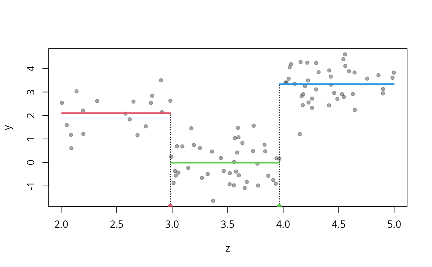
plot(os, "z", col=2:4) #plot the effect of z