Plot method for segmented objects

Takes a fitted segmented object returned by segmented() and plots (or adds) the fitted broken-line relationship for the selected segmented term.

Usage

# S3 method for class 'segmented'
plot(x, term, add=FALSE, res=FALSE, conf.level=0, interc=TRUE, link=TRUE, 
    res.col=grey(.15, alpha = .4), rev.sgn=FALSE, const=NULL, shade=FALSE, rug=!add, 
    dens.rug=FALSE, dens.col = grey(0.8), transf=I, isV=FALSE, is=FALSE, var.diff=FALSE, 
    p.df="p", .vcov=NULL, .coef=NULL, prev.trend=FALSE, smoos=NULL, hide.zeros=FALSE, 
    leg="topleft", psi.lines=FALSE, ...)

Arguments

x: a fitted segmented object.
term: Numerical or character to indicate the segmented variable having the piece-wise relationship to be plotted. If there is a single segmented variable in the fitted model x, term can be omitted. If vector, multiple segmented lines will be drawn on the same plot.
add: when TRUE the fitted lines are added to the current device.
res: when TRUE the fitted lines are plotted along with corresponding partial residuals. See Details.
conf.level: If greater than zero, it means the confidence level at which the pointwise confidence itervals have to be plotted.
interc: If TRUE the computed segmented components include the model intercept (if it exists).
link: when TRUE (default), the fitted lines are plotted on the link scale, otherwise they are tranformed on the response scale before plotting. Ignored for linear segmented fits.
res.col: when res=TRUE it means the color of the points representing the partial residuals.
rev.sgn: when TRUE it is assumed that current term is `minus' the actual segmented variable, therefore the sign is reversed before plotting. This is useful when a null-constraint has been set on the last slope.
const: constant to add to each fitted segmented relationship (on the scale of the linear predictor) before plotting. If const=NULL and the fit includes a segmented interaction term (obtained via seg(..,by) in the formula), the group-specific intercept is included.
shade: if TRUE and conf.level>0 it produces shaded regions (in grey color) for the pointwise confidence intervals embracing the fitted segmented line.
rug: when TRUE the covariate values are displayed as a rug plot at the foot of the plot. Default is to !add.
dens.rug: when TRUE then smooth covariate distribution is plotted on the x-axis.
dens.col: if dens.rug=TRUE, it means the colour to be used to plot the density.

transf: A possible function to convert the fitted values before plotting. It is only effective if res=FALSE. If res=TRUE any transformation is ignored.
isV: logical value (to be passed to broken.line). Ignored if conf.level=0
is: logical value (to be passed to broken.line) indicating if the covariance matrix based on the induced smoothing should be used. Ignored if conf.level=0
var.diff: logical value to be passed to summary.segmented to compute dthe standard errors of fitted values (if conf.level>0).
p.df: degrees of freedom when var.diff=TRUE, see summary.segmented
.vcov: The full covariance matrix of estimates to be used when conf.level>0. If unspecified (i.e. NULL), the covariance matrix is computed internally by the function vcov.segmented.
.coef: The regression parameter estimates. If unspecified (i.e. NULL), it is computed internally by coef().
prev.trend: logical. If TRUE dashed lines corresponding to the `previous' trends (i.e. the trends if the breakpoints would not have occurred) are also drawn.
smoos: logical, indicating if the residuals (provided that res=TRUE) will be drawn using a smoothed scatterplot. If NULL (default) the smoothed scatterplot will be employed when the number of observation is larger than 10000.
hide.zeros: logical, indicating if the residuals (provided that res=TRUE) corresponding to the covariate zero values should be deleted. Useful when the fit includes an interaction term in the formula, such as seg(.., by=..), and the zeros in covariates indicate units in other groups.
leg: If the plot refers to segmented relationships in groups, i.e. term has been specified as a vector, a legend is placed at the specified leg position. Put NA not to draw the legend.
psi.lines: if TRUE vertical lines corresponding to the estimated breakpoints are also drawn. Ignored if term is not a vector.
...: other graphics parameters to pass to plotting commands: `col', `lwd' and `lty' (that can be vectors and are recycled if necessary, see the example below) for the fitted piecewise lines; `ylab', `xlab', `main', `sub', `cex.axis', `cex.lab', `xlim' and `ylim' when a new plot is produced (i.e. when add=FALSE); `pch' and `cex' for the partial residuals (when res=TRUE, res.col is for the color); col.shade for the shaded regions (provided that shade=TRUE and conf.level>0).

Details

Produces (or adds to the current device) the fitted segmented relationship between the response and the selected term. If the fitted model includes just a single `segmented' variable, term may be omitted.
The partial residuals are computed as `fitted + residuals', where `fitted' are the fitted values of the segmented relationship relevant to the covariate specified in term. Notice that for GLMs the residuals are the response residuals if link=FALSE and the working residuals if link=TRUE.

Value

None.

Author

Vito M. R. Muggeo

Note

For models with offset, partial residuals on the response scale are not defined. Thus plot.segmented does not work when link=FALSE, res=TRUE, and the fitted model includes an offset.
When term is a vector and multiple segmented relationships are being drawn on the same plot, col and res.col can be vectors. Also pch, cex, lty, and lwd can be vectors, if specified.

Examples

set.seed(1234)
z<-runif(100)
y<-rpois(100,exp(2+1.8*pmax(z-.6,0)))
o<-glm(y~z,family=poisson)
o.seg<-segmented(o) #single segmented covariate and one breakpoint: 'seg.Z' and 'psi' can be omitted
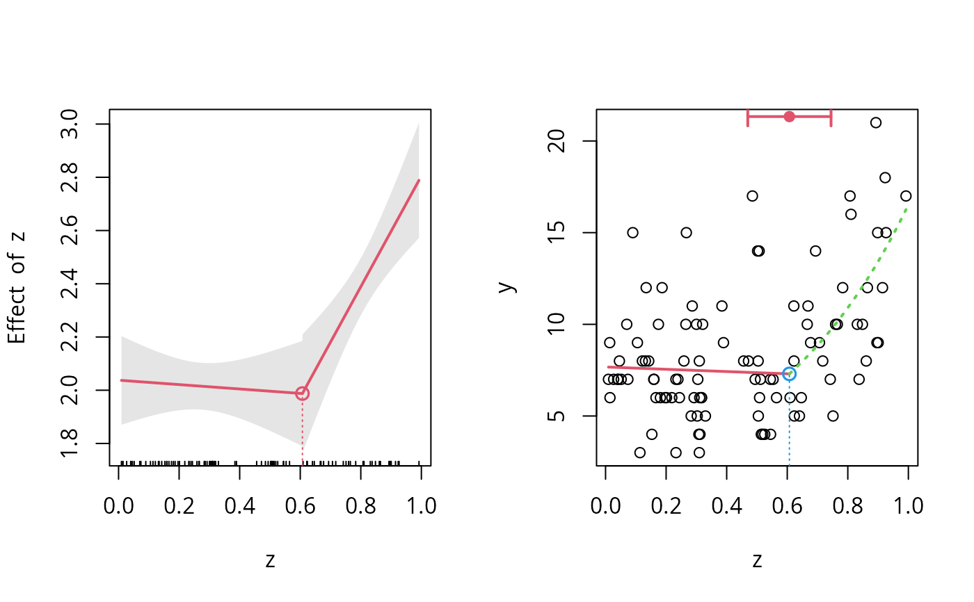
par(mfrow=c(1,2))
plot(o.seg, conf.level=0.95, shade=TRUE)
points(o.seg, link=TRUE, col=2)
## new plot
plot(z,y)
## add the fitted lines using different colors and styles..
plot(o.seg,add=TRUE,link=FALSE,lwd=2,col=2:3, lty=c(1,3))
lines(o.seg,col=2,pch=19,bottom=FALSE,lwd=2) #for the CI for the breakpoint
points(o.seg,col=4, link=FALSE)

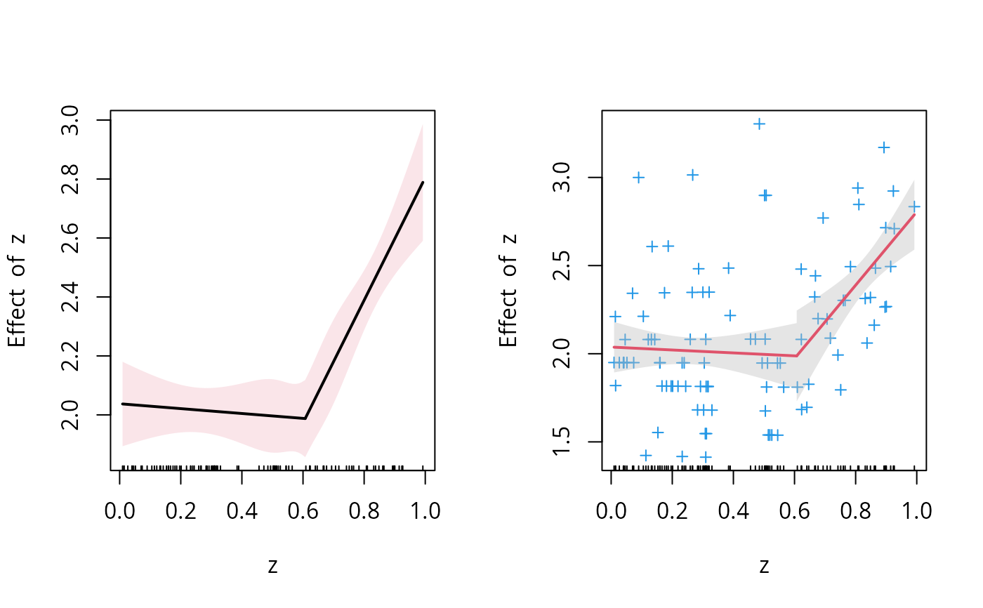
## using the options 'is', 'isV', 'shade' and 'col.shade'.
par(mfrow=c(1,2))
plot(o.seg, conf.level=.9, is=TRUE, isV=TRUE, col=1, shade = TRUE, col.shade=2)
plot(o.seg, conf.level=.9, is=TRUE, isV=FALSE, col=2, shade = TRUE, res=TRUE, res.col=4, pch=3)