meanCenter
meanCenter.RdmeanCenter selectively centers or standarizes variables in a regression model.
Usage
meanCenter(
  model,
  centerOnlyInteractors = TRUE,
  centerDV = FALSE,
  standardize = FALSE,
  terms = NULL
)

# Default S3 method
meanCenter(
  model,
  centerOnlyInteractors = TRUE,
  centerDV = FALSE,
  standardize = FALSE,
  terms = NULL
)
Arguments
- model
a fitted regression model (presumably from lm)
- centerOnlyInteractors
Default TRUE. If FALSE, all numeric predictors in the regression data frame are centered before the regression is conducted.
- centerDV
Default FALSE. Should the dependent variable be centered? Do not set this option to TRUE unless the dependent variable is a numeric variable. Otherwise, it is an error.
- standardize
Default FALSE. Instead of simply mean-centering the variables, should they also be "standardized" by first mean-centering and then dividing by the estimated standard deviation.
- terms
Optional. A vector of variable names to be centered. Supplying this argument will stop meanCenter from searching for interaction terms that might need to be centered.
Value
A regression model of the same type as the input model, with attributes representing the names of the centered variables.
Details
Works with "lm" class objects, objects estimated by glm(). This
centers some or all of the the predictors and then re-fits the
original model with the new variables. This is a convenience to
researchers who are often urged to center their predictors. This
is sometimes suggested as a way to ameliorate multi-collinearity
in models that include interaction terms (Aiken and West, 1991;
Cohen, et al 2002). Mean-centering may enhance interpretation of
the regression intercept, but it actually does not help with
multicollinearity. (Echambadi and Hess, 2007). This function
facilitates comparison of mean-centered models with others by
calculating centered variables. The defaults will cause a
regression's numeric interactive variables to be mean
centered. Variations on the arguments are discussed in details.
Suppose the user's formula that fits the original model is
m1 <- lm(y ~ x1*x2 + x3 + x4, data = dat). The fitted model
will include estimates for predictors x1, x2,
x1:x2, x3 and x4. By default,
meanCenter(m1) scans the output to see if there are
interaction terms of the form x1:x2. If so, then x1 and x2
are replaced by centered versions (m1-mean(m1)) and
(m2-mean(m2)). The model is re-estimated with those new variables.
model (the main effect and the interaction). The resulting thing
is "just another regression model", which can be analyzed or
plotted like any R regression object.
The user can claim control over which variables are centered in
several ways. Most directly, by specifying a vector of variable
names, the user can claim direct control. For example, the
argument terms=c("x1","x2","x3") would cause 3 predictors
to be centered. If one wants all predictors to be centered, the
argument centerOnlyInteractors should be set to
FALSE. Please note, this WILL NOT center factor variables. But it
will find all numeric predictors and center them.
The dependent variable will not be centered, unless the user explicitly requests it by setting centerDV = TRUE.
As an additional convenience to the user, the argument
standardize = TRUE can be used. This will divide each
centered variable by its observed standard deviation. For people
who like standardized regression, I suggest this is a better
approach than the standardize function (which is brain-dead
in the style of SPSS). meanCenter with standardize = TRUE
will only try to standardize the numeric predictors.
To be completely clear, I believe mean-centering is not helpful with the multicollinearity problem. It doesn't help, it doesn't hurt. Only a misunderstanding leads its proponents to claim otherwise. This is emphasized in the vignette "rockchalk" that is distributed with this package.
References
Aiken, L. S. and West, S.G. (1991). Multiple Regression: Testing and Interpreting Interactions. Newbury Park, Calif: Sage Publications.
Cohen, J., Cohen, P., West, S. G., and Aiken, L. S. (2002). Applied Multiple Regression/Correlation Analysis for the Behavioral Sciences (Third.). Routledge Academic.
Echambadi, R., and Hess, J. D. (2007). Mean-Centering Does Not Alleviate Collinearity Problems in Moderated Multiple Regression Models. Marketing Science, 26(3), 438-445.
Author
Paul E. Johnson pauljohn@ku.edu
Examples
library(rockchalk)
N <- 100
dat <- genCorrelatedData(N = N, means = c(100, 200), sds = c(20, 30),
rho = 0.4, stde = 10)
dat$x3 <- rnorm(100, m = 40, s = 4)
m1 <- lm(y ~ x1 * x2 + x3, data = dat)
summary(m1)
#>
#> Call:
#> lm(formula = y ~ x1 * x2 + x3, data = dat)
#>
#> Residuals:
#> Min 1Q Median 3Q Max
#> -23.8218 -5.2486 0.2155 7.2012 20.0603
#>
#> Coefficients:
#> Estimate Std. Error t value Pr(>|t|)
#> (Intercept) -4.303276 32.843988 -0.131 0.8960
#> x1 0.488960 0.311581 1.569 0.1199
#> x2 0.361707 0.163582 2.211 0.0294 *
#> x3 -0.588533 0.254145 -2.316 0.0227 *
#> x1:x2 -0.001606 0.001517 -1.059 0.2924
#> ---
#> Signif. codes: 0 ‘***’ 0.001 ‘**’ 0.01 ‘*’ 0.05 ‘.’ 0.1 ‘ ’ 1
#>
#> Residual standard error: 10.07 on 95 degrees of freedom
#> Multiple R-squared: 0.454, Adjusted R-squared: 0.431
#> F-statistic: 19.74 on 4 and 95 DF, p-value: 7.441e-12
#>
mcDiagnose(m1)
#> The following auxiliary models are being estimated and returned in a list:
#> x1 ~ x2 + x3 + `x1:x2`
#> x2 ~ x1 + x3 + `x1:x2`
#> x3 ~ x1 + x2 + `x1:x2`
#> `x1:x2` ~ x1 + x2 + x3
#>
#> R_j Squares of auxiliary models
#> x1 x2 x3 x1:x2
#> 0.97563832 0.96106395 0.03126714 0.98978825
#> The Corresponding VIF, 1/(1-R_j^2)
#> x1 x2 x3 x1:x2
#> 41.048075 25.683139 1.032276 97.926367
#> Bivariate Pearson Correlations for design matrix
#> x1 x2 x3 x1:x2
#> x1 1.00 0.53 -0.10 0.90
#> x2 0.53 1.00 -0.11 0.83
#> x3 -0.10 -0.11 1.00 -0.13
#> x1:x2 0.90 0.83 -0.13 1.00
m1c <- meanCenter(m1)
summary(m1c)
#> These variables were mean-centered before any transformations were made on the design matrix.
#> [1] "x1c" "x2c"
#> The centers and scale factors were
#> x1c x2c
#> mean 100.6557 199.8943
#> scale 1.0000 1.0000
#> The summary statistics of the variables in the design matrix (after centering).
#> mean std.dev.
#> y 60.8218 13.3553
#> x1c 0.0000 20.8199
#> x2c 0.0000 31.3683
#> x3 39.9794 4.0478
#> x1c:x2c 339.9254 693.9223
#>
#> The following results were produced from:
#> meanCenter.default(model = m1)
#>
#> Call:
#> lm(formula = y ~ x1c * x2c + x3, data = stddat)
#>
#> Residuals:
#> Min 1Q Median 3Q Max
#> -23.8218 -5.2486 0.2155 7.2012 20.0603
#>
#> Coefficients:
#> Estimate Std. Error t value Pr(>|t|)
#> (Intercept) 84.896978 10.290790 8.250 8.93e-13 ***
#> x1c 0.167870 0.057324 2.928 0.00426 **
#> x2c 0.200024 0.038560 5.187 1.20e-06 ***
#> x3 -0.588533 0.254145 -2.316 0.02272 *
#> x1c:x2c -0.001606 0.001517 -1.059 0.29240
#> ---
#> Signif. codes: 0 ‘***’ 0.001 ‘**’ 0.01 ‘*’ 0.05 ‘.’ 0.1 ‘ ’ 1
#>
#> Residual standard error: 10.07 on 95 degrees of freedom
#> Multiple R-squared: 0.454, Adjusted R-squared: 0.431
#> F-statistic: 19.74 on 4 and 95 DF, p-value: 7.441e-12
#>
mcDiagnose(m1c)
#> The following auxiliary models are being estimated and returned in a list:
#> x1c ~ x2c + x3 + `x1c:x2c`
#> x2c ~ x1c + x3 + `x1c:x2c`
#> x3 ~ x1c + x2c + `x1c:x2c`
#> `x1c:x2c` ~ x1c + x2c + x3
#>
#> R_j Squares of auxiliary models
#> x1c x2c x3 x1c:x2c
#> 0.28026276 0.29926156 0.03126714 0.07505970
#> The Corresponding VIF, 1/(1-R_j^2)
#> x1c x2c x3 x1c:x2c
#> 1.389396 1.427066 1.032276 1.081151
#> Bivariate Pearson Correlations for design matrix
#> x1c x2c x3 x1c:x2c
#> x1c 1.00 0.53 -0.10 0.17
#> x2c 0.53 1.00 -0.11 0.24
#> x3 -0.10 -0.11 1.00 -0.16
#> x1c:x2c 0.17 0.24 -0.16 1.00
m2 <- lm(y ~ x1 * x2 + x3, data = dat)
summary(m2)
#>
#> Call:
#> lm(formula = y ~ x1 * x2 + x3, data = dat)
#>
#> Residuals:
#> Min 1Q Median 3Q Max
#> -23.8218 -5.2486 0.2155 7.2012 20.0603
#>
#> Coefficients:
#> Estimate Std. Error t value Pr(>|t|)
#> (Intercept) -4.303276 32.843988 -0.131 0.8960
#> x1 0.488960 0.311581 1.569 0.1199
#> x2 0.361707 0.163582 2.211 0.0294 *
#> x3 -0.588533 0.254145 -2.316 0.0227 *
#> x1:x2 -0.001606 0.001517 -1.059 0.2924
#> ---
#> Signif. codes: 0 ‘***’ 0.001 ‘**’ 0.01 ‘*’ 0.05 ‘.’ 0.1 ‘ ’ 1
#>
#> Residual standard error: 10.07 on 95 degrees of freedom
#> Multiple R-squared: 0.454, Adjusted R-squared: 0.431
#> F-statistic: 19.74 on 4 and 95 DF, p-value: 7.441e-12
#>
mcDiagnose(m2)
#> The following auxiliary models are being estimated and returned in a list:
#> x1 ~ x2 + x3 + `x1:x2`
#> x2 ~ x1 + x3 + `x1:x2`
#> x3 ~ x1 + x2 + `x1:x2`
#> `x1:x2` ~ x1 + x2 + x3
#>
#> R_j Squares of auxiliary models
#> x1 x2 x3 x1:x2
#> 0.97563832 0.96106395 0.03126714 0.98978825
#> The Corresponding VIF, 1/(1-R_j^2)
#> x1 x2 x3 x1:x2
#> 41.048075 25.683139 1.032276 97.926367
#> Bivariate Pearson Correlations for design matrix
#> x1 x2 x3 x1:x2
#> x1 1.00 0.53 -0.10 0.90
#> x2 0.53 1.00 -0.11 0.83
#> x3 -0.10 -0.11 1.00 -0.13
#> x1:x2 0.90 0.83 -0.13 1.00
m2c <- meanCenter(m2, standardize = TRUE)
summary(m2c)
#> These variables were mean-centered before any transformations were made on the design matrix.
#> [1] "x1cs" "x2cs"
#> The centers and scale factors were
#> x1cs x2cs
#> mean 100.65566 199.89431
#> scale 20.81994 31.36831
#> The summary statistics of the variables in the design matrix (after centering).
#> mean std.dev.
#> y 60.82176 13.35527
#> x1cs 0.00000 1.00000
#> x2cs 0.00000 1.00000
#> x3 39.97940 4.04781
#> x1cs:x2cs 0.52049 1.06253
#>
#> The following results were produced from:
#> meanCenter.default(model = m2, standardize = TRUE)
#>
#> Call:
#> lm(formula = y ~ x1cs * x2cs + x3, data = stddat)
#>
#> Residuals:
#> Min 1Q Median 3Q Max
#> -23.8218 -5.2486 0.2155 7.2012 20.0603
#>
#> Coefficients:
#> Estimate Std. Error t value Pr(>|t|)
#> (Intercept) 84.8970 10.2908 8.250 8.93e-13 ***
#> x1cs 3.4950 1.1935 2.928 0.00426 **
#> x2cs 6.2744 1.2096 5.187 1.20e-06 ***
#> x3 -0.5885 0.2541 -2.316 0.02272 *
#> x1cs:x2cs -1.0491 0.9908 -1.059 0.29240
#> ---
#> Signif. codes: 0 ‘***’ 0.001 ‘**’ 0.01 ‘*’ 0.05 ‘.’ 0.1 ‘ ’ 1
#>
#> Residual standard error: 10.07 on 95 degrees of freedom
#> Multiple R-squared: 0.454, Adjusted R-squared: 0.431
#> F-statistic: 19.74 on 4 and 95 DF, p-value: 7.441e-12
#>
mcDiagnose(m2c)
#> The following auxiliary models are being estimated and returned in a list:
#> x1cs ~ x2cs + x3 + `x1cs:x2cs`
#> x2cs ~ x1cs + x3 + `x1cs:x2cs`
#> x3 ~ x1cs + x2cs + `x1cs:x2cs`
#> `x1cs:x2cs` ~ x1cs + x2cs + x3
#>
#> R_j Squares of auxiliary models
#> x1cs x2cs x3 x1cs:x2cs
#> 0.28026276 0.29926156 0.03126714 0.07505970
#> The Corresponding VIF, 1/(1-R_j^2)
#> x1cs x2cs x3 x1cs:x2cs
#> 1.389396 1.427066 1.032276 1.081151
#> Bivariate Pearson Correlations for design matrix
#> x1cs x2cs x3 x1cs:x2cs
#> x1cs 1.00 0.53 -0.10 0.17
#> x2cs 0.53 1.00 -0.11 0.24
#> x3 -0.10 -0.11 1.00 -0.16
#> x1cs:x2cs 0.17 0.24 -0.16 1.00
m2c2 <- meanCenter(m2, centerOnlyInteractors = FALSE)
summary(m2c2)
#> These variables were mean-centered before any transformations were made on the design matrix.
#> [1] "x1c" "x2c" "x3c"
#> The centers and scale factors were
#> x1c x2c x3c
#> mean 100.6557 199.8943 39.9794
#> scale 1.0000 1.0000 1.0000
#> The summary statistics of the variables in the design matrix (after centering).
#> mean std.dev.
#> y 60.8218 13.3553
#> x1c 0.0000 20.8199
#> x2c 0.0000 31.3683
#> x3c 0.0000 4.0478
#> x1c:x2c 339.9254 693.9223
#>
#> The following results were produced from:
#> meanCenter.default(model = m2, centerOnlyInteractors = FALSE)
#>
#> Call:
#> lm(formula = y ~ x1c * x2c + x3c, data = stddat)
#>
#> Residuals:
#> Min 1Q Median 3Q Max
#> -23.8218 -5.2486 0.2155 7.2012 20.0603
#>
#> Coefficients:
#> Estimate Std. Error t value Pr(>|t|)
#> (Intercept) 61.367781 1.131776 54.223 < 2e-16 ***
#> x1c 0.167870 0.057324 2.928 0.00426 **
#> x2c 0.200024 0.038560 5.187 1.2e-06 ***
#> x3c -0.588533 0.254145 -2.316 0.02272 *
#> x1c:x2c -0.001606 0.001517 -1.059 0.29240
#> ---
#> Signif. codes: 0 ‘***’ 0.001 ‘**’ 0.01 ‘*’ 0.05 ‘.’ 0.1 ‘ ’ 1
#>
#> Residual standard error: 10.07 on 95 degrees of freedom
#> Multiple R-squared: 0.454, Adjusted R-squared: 0.431
#> F-statistic: 19.74 on 4 and 95 DF, p-value: 7.441e-12
#>
m2c3 <- meanCenter(m2, centerOnlyInteractors = FALSE, centerDV = TRUE)
summary(m2c3)
#> These variables were mean-centered before any transformations were made on the design matrix.
#> [1] "yc" "x1c" "x2c" "x3c"
#> The centers and scale factors were
#> yc x1c x2c x3c
#> mean 60.82176 100.6557 199.8943 39.9794
#> scale 1.00000 1.0000 1.0000 1.0000
#> The summary statistics of the variables in the design matrix (after centering).
#> mean std.dev.
#> yc 0.0000 13.3553
#> x1c 0.0000 20.8199
#> x2c 0.0000 31.3683
#> x3c 0.0000 4.0478
#> x1c:x2c 339.9254 693.9223
#>
#> The following results were produced from:
#> meanCenter.default(model = m2, centerOnlyInteractors = FALSE,
#> centerDV = TRUE)
#>
#> Call:
#> lm(formula = yc ~ x1c * x2c + x3c, data = stddat)
#>
#> Residuals:
#> Min 1Q Median 3Q Max
#> -23.8218 -5.2486 0.2155 7.2012 20.0603
#>
#> Coefficients:
#> Estimate Std. Error t value Pr(>|t|)
#> (Intercept) 0.546023 1.131776 0.482 0.63060
#> x1c 0.167870 0.057324 2.928 0.00426 **
#> x2c 0.200024 0.038560 5.187 1.2e-06 ***
#> x3c -0.588533 0.254145 -2.316 0.02272 *
#> x1c:x2c -0.001606 0.001517 -1.059 0.29240
#> ---
#> Signif. codes: 0 ‘***’ 0.001 ‘**’ 0.01 ‘*’ 0.05 ‘.’ 0.1 ‘ ’ 1
#>
#> Residual standard error: 10.07 on 95 degrees of freedom
#> Multiple R-squared: 0.454, Adjusted R-squared: 0.431
#> F-statistic: 19.74 on 4 and 95 DF, p-value: 7.441e-12
#>
dat <- genCorrelatedData(N = N, means = c(100, 200), sds = c(20, 30),
rho = 0.4, stde = 10)
dat$x3 <- rnorm(100, m = 40, s = 4)
dat$x3 <- gl(4, 25, labels = c("none", "some", "much", "total"))
m3 <- lm(y ~ x1 * x2 + x3, data = dat)
summary(m3)
#>
#> Call:
#> lm(formula = y ~ x1 * x2 + x3, data = dat)
#>
#> Residuals:
#> Min 1Q Median 3Q Max
#> -27.396 -9.117 1.768 9.149 28.906
#>
#> Coefficients:
#> Estimate Std. Error t value Pr(>|t|)
#> (Intercept) -8.749e-01 4.448e+01 -0.020 0.984
#> x1 2.531e-01 4.352e-01 0.582 0.562
#> x2 1.683e-01 2.312e-01 0.728 0.468
#> x3some -1.115e+00 3.394e+00 -0.329 0.743
#> x3much -5.139e-01 3.381e+00 -0.152 0.880
#> x3total 3.965e-01 3.454e+00 0.115 0.909
#> x1:x2 8.575e-05 2.224e-03 0.039 0.969
#>
#> Residual standard error: 11.94 on 93 degrees of freedom
#> Multiple R-squared: 0.3645, Adjusted R-squared: 0.3235
#> F-statistic: 8.89 on 6 and 93 DF, p-value: 1.153e-07
#>
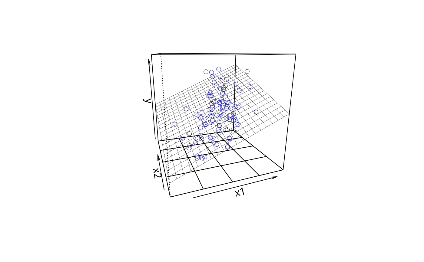
## visualize, for fun
plotPlane(m3, "x1", "x2")
 m3c1 <- meanCenter(m3)
summary(m3c1)
#> These variables were mean-centered before any transformations were made on the design matrix.
#> [1] "x1c" "x2c"
#> The centers and scale factors were
#> x1c x2c
#> mean 98.19437 197.2157
#> scale 1.00000 1.0000
#> The summary statistics of the variables in the design matrix (after centering).
#> mean std.dev.
#> y 58.5421 14.5225
#> x1c 0.0000 20.6578
#> x2c 0.0000 28.3323
#> x3some 0.2500 0.4352
#> x3much 0.2500 0.4352
#> x3total 0.2500 0.4352
#> x1c:x2c 220.0519 551.8863
#>
#> The following results were produced from:
#> meanCenter.default(model = m3)
#>
#> Call:
#> lm(formula = y ~ x1c * x2c + x3, data = stddat)
#>
#> Residuals:
#> Min 1Q Median 3Q Max
#> -27.396 -9.117 1.768 9.149 28.906
#>
#> Coefficients:
#> Estimate Std. Error t value Pr(>|t|)
#> (Intercept) 5.883e+01 2.441e+00 24.105 < 2e-16 ***
#> x1c 2.700e-01 6.451e-02 4.186 6.45e-05 ***
#> x2c 1.767e-01 4.677e-02 3.779 0.000278 ***
#> x3some -1.115e+00 3.394e+00 -0.329 0.743240
#> x3much -5.139e-01 3.381e+00 -0.152 0.879516
#> x3total 3.965e-01 3.454e+00 0.115 0.908858
#> x1c:x2c 8.575e-05 2.224e-03 0.039 0.969321
#> ---
#> Signif. codes: 0 ‘***’ 0.001 ‘**’ 0.01 ‘*’ 0.05 ‘.’ 0.1 ‘ ’ 1
#>
#> Residual standard error: 11.94 on 93 degrees of freedom
#> Multiple R-squared: 0.3645, Adjusted R-squared: 0.3235
#> F-statistic: 8.89 on 6 and 93 DF, p-value: 1.153e-07
#>
## Not exactly the same as a "standardized" regression because the
## interactive variables are centered in the model frame,
## and the term "x1:x2" is never centered again.
m3c2 <- meanCenter(m3, centerDV = TRUE,
centerOnlyInteractors = FALSE, standardize = TRUE)
summary(m3c2)
#> These variables were mean-centered before any transformations were made on the design matrix.
#> [1] "ycs" "x1cs" "x2cs"
#> The centers and scale factors were
#> ycs x1cs x2cs
#> mean 58.54205 98.19437 197.21566
#> scale 14.52252 20.65785 28.33228
#> The summary statistics of the variables in the design matrix (after centering).
#> mean std.dev.
#> ycs 0.0000000 1.0000000
#> x1cs 0.0000000 1.0000000
#> x2cs 0.0000000 1.0000000
#> x3some 0.2500000 0.4351941
#> x3much 0.2500000 0.4351941
#> x3total 0.2500000 0.4351941
#> x1cs:x2cs 0.3759746 0.9429379
#>
#> The following results were produced from:
#> meanCenter.default(model = m3, centerOnlyInteractors = FALSE,
#> centerDV = TRUE, standardize = TRUE)
#>
#> Call:
#> lm(formula = ycs ~ x1cs * x2cs + x3, data = stddat)
#>
#> Residuals:
#> Min 1Q Median 3Q Max
#> -1.8864 -0.6278 0.1217 0.6300 1.9904
#>
#> Coefficients:
#> Estimate Std. Error t value Pr(>|t|)
#> (Intercept) 0.019920 0.168058 0.119 0.905905
#> x1cs 0.384099 0.091764 4.186 6.45e-05 ***
#> x2cs 0.344769 0.091245 3.779 0.000278 ***
#> x3some -0.076788 0.233724 -0.329 0.743240
#> x3much -0.035387 0.232807 -0.152 0.879516
#> x3total 0.027300 0.237820 0.115 0.908858
#> x1cs:x2cs 0.003456 0.089613 0.039 0.969321
#> ---
#> Signif. codes: 0 ‘***’ 0.001 ‘**’ 0.01 ‘*’ 0.05 ‘.’ 0.1 ‘ ’ 1
#>
#> Residual standard error: 0.8225 on 93 degrees of freedom
#> Multiple R-squared: 0.3645, Adjusted R-squared: 0.3235
#> F-statistic: 8.89 on 6 and 93 DF, p-value: 1.153e-07
#>
m3st <- standardize(m3)
summary(m3st)
#> All variables in the model matrix and the dependent variable
#> were centered. The centered variables have the letter "s" appended to their
#> non-centered counterparts, even constructed
#> variables like `x1:x2` and poly(x1,2). We agree, that's probably
#> ill-advised, but you asked for it by running standardize().
#>
#> The rockchalk function meanCenter is a smarter option, probably.
#>
#> The summary statistics of the variables in the design matrix.
#> mean std.dev.
#> ys 0 1
#> x1s 0 1
#> x2s 0 1
#> x3somes 0 1
#> x3muchs 0 1
#> x3totals 0 1
#> `x1:x2s` 0 1
#>
#> Call:
#> lm(formula = ys ~ -1 + x1s + x2s + x3somes + x3muchs + x3totals +
#> `x1:x2s`, data = stddat)
#>
#> Residuals:
#> Min 1Q Median 3Q Max
#> -1.8864 -0.6278 0.1217 0.6300 1.9904
#>
#> Coefficients:
#> Estimate Std. Error t value Pr(>|t|)
#> x1s 0.36004 0.61577 0.585 0.560
#> x2s 0.32834 0.44864 0.732 0.466
#> x3somes -0.03342 0.10117 -0.330 0.742
#> x3muchs -0.01540 0.10078 -0.153 0.879
#> x3totals 0.01188 0.10295 0.115 0.908
#> `x1:x2s` 0.03408 0.87894 0.039 0.969
#>
#> Residual standard error: 0.8181 on 94 degrees of freedom
#> Multiple R-squared: 0.3645, Adjusted R-squared: 0.3239
#> F-statistic: 8.985 on 6 and 94 DF, p-value: 9.378e-08
#>
## Make a bigger dataset to see effects better
N <- 500
dat <- genCorrelatedData(N = N, means = c(200,200), sds = c(60,30),
rho = 0.2, stde = 10)
dat$x3 <- rnorm(100, m = 40, s = 4)
dat$x3 <- gl(4, 25, labels = c("none", "some", "much", "total"))
dat$y2 <- with(dat,
0.4 - 0.15 * x1 + 0.04 * x1^2 -
drop(contrasts(dat$x3)[dat$x3, ] %*% c(-1.9, 0, 5.1)) +
1000* rnorm(nrow(dat)))
dat$y2 <- drop(dat$y2)
m4literal <- lm(y2 ~ x1 + I(x1*x1) + x2 + x3, data = dat)
summary(m4literal)
#>
#> Call:
#> lm(formula = y2 ~ x1 + I(x1 * x1) + x2 + x3, data = dat)
#>
#> Residuals:
#> Min 1Q Median 3Q Max
#> -2512.0 -723.1 -12.7 620.6 3291.0
#>
#> Coefficients:
#> Estimate Std. Error t value Pr(>|t|)
#> (Intercept) 382.94721 445.35389 0.860 0.390
#> x1 -1.59014 3.71343 -0.428 0.669
#> I(x1 * x1) 0.04269 0.00905 4.717 3.11e-06 ***
#> x2 -1.40434 1.50847 -0.931 0.352
#> x3some -52.23259 124.90769 -0.418 0.676
#> x3much 65.45299 125.16971 0.523 0.601
#> x3total 55.41979 124.83644 0.444 0.657
#> ---
#> Signif. codes: 0 ‘***’ 0.001 ‘**’ 0.01 ‘*’ 0.05 ‘.’ 0.1 ‘ ’ 1
#>
#> Residual standard error: 985.6 on 493 degrees of freedom
#> Multiple R-squared: 0.4729, Adjusted R-squared: 0.4664
#> F-statistic: 73.7 on 6 and 493 DF, p-value: < 2.2e-16
#>
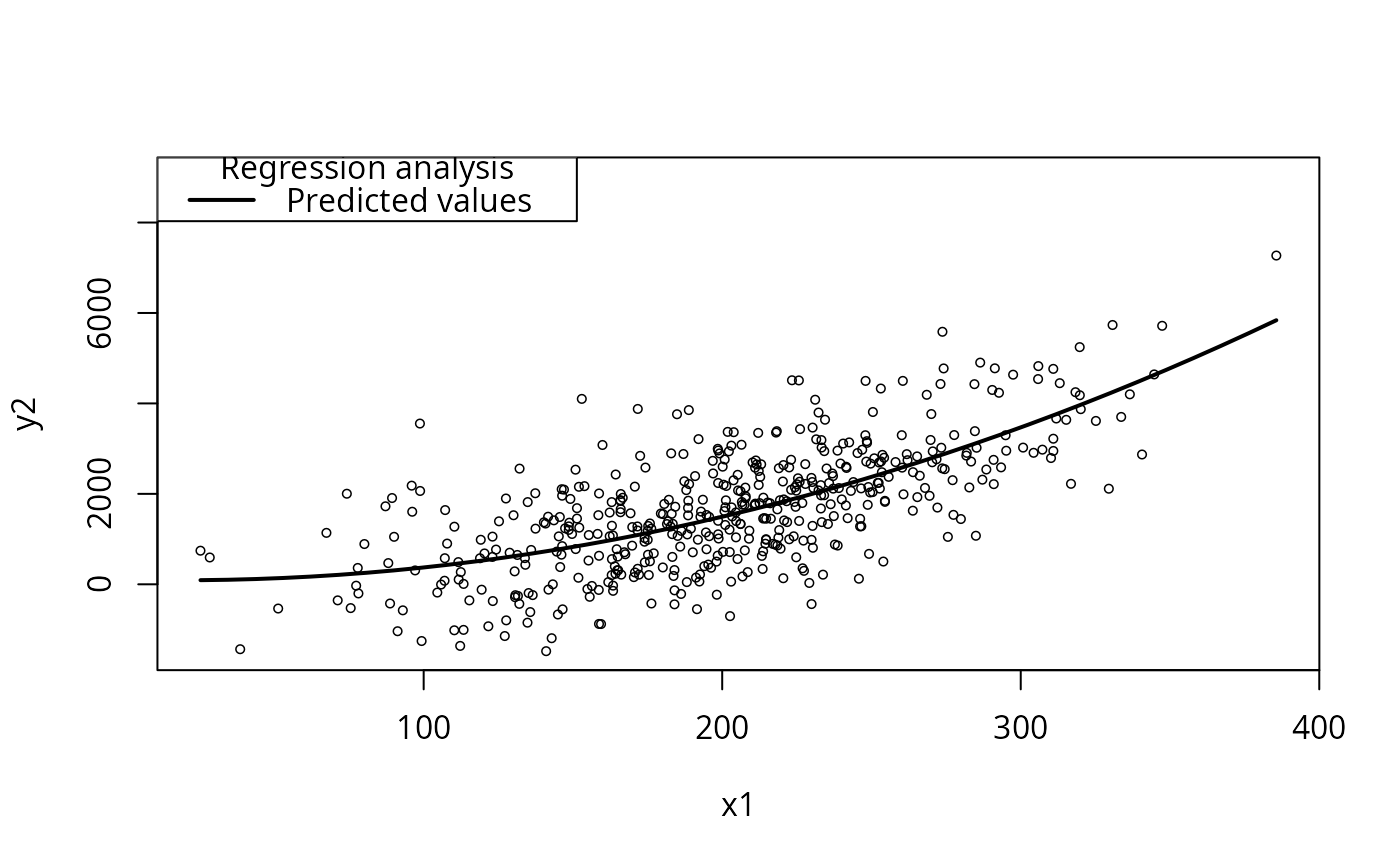
plotCurves(m4literal, plotx="x1")
m3c1 <- meanCenter(m3)
summary(m3c1)
#> These variables were mean-centered before any transformations were made on the design matrix.
#> [1] "x1c" "x2c"
#> The centers and scale factors were
#> x1c x2c
#> mean 98.19437 197.2157
#> scale 1.00000 1.0000
#> The summary statistics of the variables in the design matrix (after centering).
#> mean std.dev.
#> y 58.5421 14.5225
#> x1c 0.0000 20.6578
#> x2c 0.0000 28.3323
#> x3some 0.2500 0.4352
#> x3much 0.2500 0.4352
#> x3total 0.2500 0.4352
#> x1c:x2c 220.0519 551.8863
#>
#> The following results were produced from:
#> meanCenter.default(model = m3)
#>
#> Call:
#> lm(formula = y ~ x1c * x2c + x3, data = stddat)
#>
#> Residuals:
#> Min 1Q Median 3Q Max
#> -27.396 -9.117 1.768 9.149 28.906
#>
#> Coefficients:
#> Estimate Std. Error t value Pr(>|t|)
#> (Intercept) 5.883e+01 2.441e+00 24.105 < 2e-16 ***
#> x1c 2.700e-01 6.451e-02 4.186 6.45e-05 ***
#> x2c 1.767e-01 4.677e-02 3.779 0.000278 ***
#> x3some -1.115e+00 3.394e+00 -0.329 0.743240
#> x3much -5.139e-01 3.381e+00 -0.152 0.879516
#> x3total 3.965e-01 3.454e+00 0.115 0.908858
#> x1c:x2c 8.575e-05 2.224e-03 0.039 0.969321
#> ---
#> Signif. codes: 0 ‘***’ 0.001 ‘**’ 0.01 ‘*’ 0.05 ‘.’ 0.1 ‘ ’ 1
#>
#> Residual standard error: 11.94 on 93 degrees of freedom
#> Multiple R-squared: 0.3645, Adjusted R-squared: 0.3235
#> F-statistic: 8.89 on 6 and 93 DF, p-value: 1.153e-07
#>
## Not exactly the same as a "standardized" regression because the
## interactive variables are centered in the model frame,
## and the term "x1:x2" is never centered again.
m3c2 <- meanCenter(m3, centerDV = TRUE,
centerOnlyInteractors = FALSE, standardize = TRUE)
summary(m3c2)
#> These variables were mean-centered before any transformations were made on the design matrix.
#> [1] "ycs" "x1cs" "x2cs"
#> The centers and scale factors were
#> ycs x1cs x2cs
#> mean 58.54205 98.19437 197.21566
#> scale 14.52252 20.65785 28.33228
#> The summary statistics of the variables in the design matrix (after centering).
#> mean std.dev.
#> ycs 0.0000000 1.0000000
#> x1cs 0.0000000 1.0000000
#> x2cs 0.0000000 1.0000000
#> x3some 0.2500000 0.4351941
#> x3much 0.2500000 0.4351941
#> x3total 0.2500000 0.4351941
#> x1cs:x2cs 0.3759746 0.9429379
#>
#> The following results were produced from:
#> meanCenter.default(model = m3, centerOnlyInteractors = FALSE,
#> centerDV = TRUE, standardize = TRUE)
#>
#> Call:
#> lm(formula = ycs ~ x1cs * x2cs + x3, data = stddat)
#>
#> Residuals:
#> Min 1Q Median 3Q Max
#> -1.8864 -0.6278 0.1217 0.6300 1.9904
#>
#> Coefficients:
#> Estimate Std. Error t value Pr(>|t|)
#> (Intercept) 0.019920 0.168058 0.119 0.905905
#> x1cs 0.384099 0.091764 4.186 6.45e-05 ***
#> x2cs 0.344769 0.091245 3.779 0.000278 ***
#> x3some -0.076788 0.233724 -0.329 0.743240
#> x3much -0.035387 0.232807 -0.152 0.879516
#> x3total 0.027300 0.237820 0.115 0.908858
#> x1cs:x2cs 0.003456 0.089613 0.039 0.969321
#> ---
#> Signif. codes: 0 ‘***’ 0.001 ‘**’ 0.01 ‘*’ 0.05 ‘.’ 0.1 ‘ ’ 1
#>
#> Residual standard error: 0.8225 on 93 degrees of freedom
#> Multiple R-squared: 0.3645, Adjusted R-squared: 0.3235
#> F-statistic: 8.89 on 6 and 93 DF, p-value: 1.153e-07
#>
m3st <- standardize(m3)
summary(m3st)
#> All variables in the model matrix and the dependent variable
#> were centered. The centered variables have the letter "s" appended to their
#> non-centered counterparts, even constructed
#> variables like `x1:x2` and poly(x1,2). We agree, that's probably
#> ill-advised, but you asked for it by running standardize().
#>
#> The rockchalk function meanCenter is a smarter option, probably.
#>
#> The summary statistics of the variables in the design matrix.
#> mean std.dev.
#> ys 0 1
#> x1s 0 1
#> x2s 0 1
#> x3somes 0 1
#> x3muchs 0 1
#> x3totals 0 1
#> `x1:x2s` 0 1
#>
#> Call:
#> lm(formula = ys ~ -1 + x1s + x2s + x3somes + x3muchs + x3totals +
#> `x1:x2s`, data = stddat)
#>
#> Residuals:
#> Min 1Q Median 3Q Max
#> -1.8864 -0.6278 0.1217 0.6300 1.9904
#>
#> Coefficients:
#> Estimate Std. Error t value Pr(>|t|)
#> x1s 0.36004 0.61577 0.585 0.560
#> x2s 0.32834 0.44864 0.732 0.466
#> x3somes -0.03342 0.10117 -0.330 0.742
#> x3muchs -0.01540 0.10078 -0.153 0.879
#> x3totals 0.01188 0.10295 0.115 0.908
#> `x1:x2s` 0.03408 0.87894 0.039 0.969
#>
#> Residual standard error: 0.8181 on 94 degrees of freedom
#> Multiple R-squared: 0.3645, Adjusted R-squared: 0.3239
#> F-statistic: 8.985 on 6 and 94 DF, p-value: 9.378e-08
#>
## Make a bigger dataset to see effects better
N <- 500
dat <- genCorrelatedData(N = N, means = c(200,200), sds = c(60,30),
rho = 0.2, stde = 10)
dat$x3 <- rnorm(100, m = 40, s = 4)
dat$x3 <- gl(4, 25, labels = c("none", "some", "much", "total"))
dat$y2 <- with(dat,
0.4 - 0.15 * x1 + 0.04 * x1^2 -
drop(contrasts(dat$x3)[dat$x3, ] %*% c(-1.9, 0, 5.1)) +
1000* rnorm(nrow(dat)))
dat$y2 <- drop(dat$y2)
m4literal <- lm(y2 ~ x1 + I(x1*x1) + x2 + x3, data = dat)
summary(m4literal)
#>
#> Call:
#> lm(formula = y2 ~ x1 + I(x1 * x1) + x2 + x3, data = dat)
#>
#> Residuals:
#> Min 1Q Median 3Q Max
#> -2512.0 -723.1 -12.7 620.6 3291.0
#>
#> Coefficients:
#> Estimate Std. Error t value Pr(>|t|)
#> (Intercept) 382.94721 445.35389 0.860 0.390
#> x1 -1.59014 3.71343 -0.428 0.669
#> I(x1 * x1) 0.04269 0.00905 4.717 3.11e-06 ***
#> x2 -1.40434 1.50847 -0.931 0.352
#> x3some -52.23259 124.90769 -0.418 0.676
#> x3much 65.45299 125.16971 0.523 0.601
#> x3total 55.41979 124.83644 0.444 0.657
#> ---
#> Signif. codes: 0 ‘***’ 0.001 ‘**’ 0.01 ‘*’ 0.05 ‘.’ 0.1 ‘ ’ 1
#>
#> Residual standard error: 985.6 on 493 degrees of freedom
#> Multiple R-squared: 0.4729, Adjusted R-squared: 0.4664
#> F-statistic: 73.7 on 6 and 493 DF, p-value: < 2.2e-16
#>
plotCurves(m4literal, plotx="x1")
 ## Superficially, there is multicollinearity (omit the intercept)
cor(model.matrix(m4literal)[ -1 , -1 ])
#> x1 I(x1 * x1) x2 x3some x3much
#> x1 1.00000000 0.979056414 0.251709996 -0.01097151 0.07610925
#> I(x1 * x1) 0.97905641 1.000000000 0.237029989 -0.01260037 0.07775549
#> x2 0.25171000 0.237029989 1.000000000 0.05048286 -0.01182650
#> x3some -0.01097151 -0.012600368 0.050482859 1.00000000 -0.33422460
#> x3much 0.07610925 0.077755489 -0.011826500 -0.33422460 1.00000000
#> x3total 0.00200490 0.004955053 0.004878339 -0.33422460 -0.33422460
#> x3total
#> x1 0.002004900
#> I(x1 * x1) 0.004955053
#> x2 0.004878339
#> x3some -0.334224599
#> x3much -0.334224599
#> x3total 1.000000000
m4literalmc <- meanCenter(m4literal, terms = "x1")
summary(m4literalmc)
#> These variables were mean-centered before any transformations were made on the design matrix.
#> [1] "x1c"
#> The centers and scale factors were
#> x1c
#> mean 201.1362
#> scale 1.0000
#> The summary statistics of the variables in the design matrix (after centering).
#> mean std.dev.
#> y2 1675.440 1349.335
#> x1c 0.000 58.674
#> I(x1c * x1c) 3435.727 4884.529
#> x2 198.387 30.312
#> x3some 0.250 0.433
#> x3much 0.250 0.433
#> x3total 0.250 0.433
#>
#> The following results were produced from:
#> meanCenter.default(model = m4literal, terms = "x1")
#>
#> Call:
#> lm(formula = y2 ~ x1c + I(x1c * x1c) + x2 + x3, data = stddat)
#>
#> Residuals:
#> Min 1Q Median 3Q Max
#> -2512.0 -723.1 -12.7 620.6 3291.0
#>
#> Coefficients:
#> Estimate Std. Error t value Pr(>|t|)
#> (Intercept) 1790.20817 312.68746 5.725 1.80e-08 ***
#> x1c 15.58325 0.78009 19.976 < 2e-16 ***
#> I(x1c * x1c) 0.04269 0.00905 4.717 3.11e-06 ***
#> x2 -1.40434 1.50847 -0.931 0.352
#> x3some -52.23259 124.90769 -0.418 0.676
#> x3much 65.45299 125.16971 0.523 0.601
#> x3total 55.41979 124.83644 0.444 0.657
#> ---
#> Signif. codes: 0 ‘***’ 0.001 ‘**’ 0.01 ‘*’ 0.05 ‘.’ 0.1 ‘ ’ 1
#>
#> Residual standard error: 985.6 on 493 degrees of freedom
#> Multiple R-squared: 0.4729, Adjusted R-squared: 0.4664
#> F-statistic: 73.7 on 6 and 493 DF, p-value: < 2.2e-16
#>
m4literalmcs <- meanCenter(m4literal, terms = "x1", standardize = TRUE)
summary(m4literalmcs)
#> These variables were mean-centered before any transformations were made on the design matrix.
#> [1] "x1cs"
#> The centers and scale factors were
#> x1cs
#> mean 201.13617
#> scale 58.67378
#> The summary statistics of the variables in the design matrix (after centering).
#> mean std.dev.
#> y2 1675.4404 1349.3349
#> x1cs 0.0000 1.0000
#> I(x1cs * x1cs) 0.9980 1.4188
#> x2 198.3866 30.3125
#> x3some 0.2500 0.4334
#> x3much 0.2500 0.4334
#> x3total 0.2500 0.4334
#>
#> The following results were produced from:
#> meanCenter.default(model = m4literal, standardize = TRUE, terms = "x1")
#>
#> Call:
#> lm(formula = y2 ~ x1cs + I(x1cs * x1cs) + x2 + x3, data = stddat)
#>
#> Residuals:
#> Min 1Q Median 3Q Max
#> -2512.0 -723.1 -12.7 620.6 3291.0
#>
#> Coefficients:
#> Estimate Std. Error t value Pr(>|t|)
#> (Intercept) 1790.208 312.687 5.725 1.80e-08 ***
#> x1cs 914.328 45.771 19.976 < 2e-16 ***
#> I(x1cs * x1cs) 146.968 31.154 4.717 3.11e-06 ***
#> x2 -1.404 1.508 -0.931 0.352
#> x3some -52.233 124.908 -0.418 0.676
#> x3much 65.453 125.170 0.523 0.601
#> x3total 55.420 124.836 0.444 0.657
#> ---
#> Signif. codes: 0 ‘***’ 0.001 ‘**’ 0.01 ‘*’ 0.05 ‘.’ 0.1 ‘ ’ 1
#>
#> Residual standard error: 985.6 on 493 degrees of freedom
#> Multiple R-squared: 0.4729, Adjusted R-squared: 0.4664
#> F-statistic: 73.7 on 6 and 493 DF, p-value: < 2.2e-16
#>
m4 <- lm(y2 ~ poly(x1, 2, raw = TRUE) + x2 + x3, data = dat)
summary(m4)
#>
#> Call:
#> lm(formula = y2 ~ poly(x1, 2, raw = TRUE) + x2 + x3, data = dat)
#>
#> Residuals:
#> Min 1Q Median 3Q Max
#> -2512.0 -723.1 -12.7 620.6 3291.0
#>
#> Coefficients:
#> Estimate Std. Error t value Pr(>|t|)
#> (Intercept) 382.94721 445.35389 0.860 0.390
#> poly(x1, 2, raw = TRUE)1 -1.59014 3.71343 -0.428 0.669
#> poly(x1, 2, raw = TRUE)2 0.04269 0.00905 4.717 3.11e-06 ***
#> x2 -1.40434 1.50847 -0.931 0.352
#> x3some -52.23259 124.90769 -0.418 0.676
#> x3much 65.45299 125.16971 0.523 0.601
#> x3total 55.41979 124.83644 0.444 0.657
#> ---
#> Signif. codes: 0 ‘***’ 0.001 ‘**’ 0.01 ‘*’ 0.05 ‘.’ 0.1 ‘ ’ 1
#>
#> Residual standard error: 985.6 on 493 degrees of freedom
#> Multiple R-squared: 0.4729, Adjusted R-squared: 0.4664
#> F-statistic: 73.7 on 6 and 493 DF, p-value: < 2.2e-16
#>
plotCurves(m4, plotx="x1")
m4mc1 <- meanCenter(m4, terms = "x1")
summary(m4mc1)
#> These variables were mean-centered before any transformations were made on the design matrix.
#> [1] "x1c"
#> The centers and scale factors were
#> x1c
#> mean 201.1362
#> scale 1.0000
#> The summary statistics of the variables in the design matrix (after centering).
#> mean std.dev.
#> y2 1675.440 1349.335
#> poly(x1c, 2, raw = TRUE)1 0.000 58.674
#> poly(x1c, 2, raw = TRUE)2 3435.727 4884.529
#> x2 198.387 30.312
#> x3some 0.250 0.433
#> x3much 0.250 0.433
#> x3total 0.250 0.433
#>
#> The following results were produced from:
#> meanCenter.default(model = m4, terms = "x1")
#>
#> Call:
#> lm(formula = y2 ~ poly(x1c, 2, raw = TRUE) + x2 + x3, data = stddat)
#>
#> Residuals:
#> Min 1Q Median 3Q Max
#> -2512.0 -723.1 -12.7 620.6 3291.0
#>
#> Coefficients:
#> Estimate Std. Error t value Pr(>|t|)
#> (Intercept) 1790.20817 312.68746 5.725 1.80e-08 ***
#> poly(x1c, 2, raw = TRUE)1 15.58325 0.78009 19.976 < 2e-16 ***
#> poly(x1c, 2, raw = TRUE)2 0.04269 0.00905 4.717 3.11e-06 ***
#> x2 -1.40434 1.50847 -0.931 0.352
#> x3some -52.23259 124.90769 -0.418 0.676
#> x3much 65.45299 125.16971 0.523 0.601
#> x3total 55.41979 124.83644 0.444 0.657
#> ---
#> Signif. codes: 0 ‘***’ 0.001 ‘**’ 0.01 ‘*’ 0.05 ‘.’ 0.1 ‘ ’ 1
#>
#> Residual standard error: 985.6 on 493 degrees of freedom
#> Multiple R-squared: 0.4729, Adjusted R-squared: 0.4664
#> F-statistic: 73.7 on 6 and 493 DF, p-value: < 2.2e-16
#>
m4mc2 <- meanCenter(m4, terms = "x1", standardize = TRUE)
summary(m4mc2)
#> These variables were mean-centered before any transformations were made on the design matrix.
#> [1] "x1cs"
#> The centers and scale factors were
#> x1cs
#> mean 201.13617
#> scale 58.67378
#> The summary statistics of the variables in the design matrix (after centering).
#> mean std.dev.
#> y2 1675.4404 1349.3349
#> poly(x1cs, 2, raw = TRUE)1 0.0000 1.0000
#> poly(x1cs, 2, raw = TRUE)2 0.9980 1.4188
#> x2 198.3866 30.3125
#> x3some 0.2500 0.4334
#> x3much 0.2500 0.4334
#> x3total 0.2500 0.4334
#>
#> The following results were produced from:
#> meanCenter.default(model = m4, standardize = TRUE, terms = "x1")
#>
#> Call:
#> lm(formula = y2 ~ poly(x1cs, 2, raw = TRUE) + x2 + x3, data = stddat)
#>
#> Residuals:
#> Min 1Q Median 3Q Max
#> -2512.0 -723.1 -12.7 620.6 3291.0
#>
#> Coefficients:
#> Estimate Std. Error t value Pr(>|t|)
#> (Intercept) 1790.208 312.687 5.725 1.80e-08 ***
#> poly(x1cs, 2, raw = TRUE)1 914.328 45.771 19.976 < 2e-16 ***
#> poly(x1cs, 2, raw = TRUE)2 146.968 31.154 4.717 3.11e-06 ***
#> x2 -1.404 1.508 -0.931 0.352
#> x3some -52.233 124.908 -0.418 0.676
#> x3much 65.453 125.170 0.523 0.601
#> x3total 55.420 124.836 0.444 0.657
#> ---
#> Signif. codes: 0 ‘***’ 0.001 ‘**’ 0.01 ‘*’ 0.05 ‘.’ 0.1 ‘ ’ 1
#>
#> Residual standard error: 985.6 on 493 degrees of freedom
#> Multiple R-squared: 0.4729, Adjusted R-squared: 0.4664
#> F-statistic: 73.7 on 6 and 493 DF, p-value: < 2.2e-16
#>
m4mc3 <- meanCenter(m4, terms = "x1", centerDV = TRUE, standardize = TRUE)
summary(m4mc3)
#> These variables were mean-centered before any transformations were made on the design matrix.
#> [1] "y2cs" "x1cs"
#> The centers and scale factors were
#> y2cs x1cs
#> mean 1675.440 201.13617
#> scale 1349.335 58.67378
#> The summary statistics of the variables in the design matrix (after centering).
#> mean std.dev.
#> y2cs 0.0000 1.00000
#> poly(x1cs, 2, raw = TRUE)1 0.0000 1.00000
#> poly(x1cs, 2, raw = TRUE)2 0.9980 1.41884
#> x2 198.3866 30.31246
#> x3some 0.2500 0.43345
#> x3much 0.2500 0.43345
#> x3total 0.2500 0.43345
#>
#> The following results were produced from:
#> meanCenter.default(model = m4, centerDV = TRUE, standardize = TRUE,
#> terms = "x1")
#>
#> Call:
#> lm(formula = y2cs ~ poly(x1cs, 2, raw = TRUE) + x2 + x3, data = stddat)
#>
#> Residuals:
#> Min 1Q Median 3Q Max
#> -1.86168 -0.53587 -0.00939 0.45992 2.43901
#>
#> Coefficients:
#> Estimate Std. Error t value Pr(>|t|)
#> (Intercept) 0.085055 0.231735 0.367 0.714
#> poly(x1cs, 2, raw = TRUE)1 0.677614 0.033921 19.976 < 2e-16 ***
#> poly(x1cs, 2, raw = TRUE)2 0.108919 0.023088 4.717 3.11e-06 ***
#> x2 -0.001041 0.001118 -0.931 0.352
#> x3some -0.038710 0.092570 -0.418 0.676
#> x3much 0.048508 0.092764 0.523 0.601
#> x3total 0.041072 0.092517 0.444 0.657
#> ---
#> Signif. codes: 0 ‘***’ 0.001 ‘**’ 0.01 ‘*’ 0.05 ‘.’ 0.1 ‘ ’ 1
#>
#> Residual standard error: 0.7305 on 493 degrees of freedom
#> Multiple R-squared: 0.4729, Adjusted R-squared: 0.4664
#> F-statistic: 73.7 on 6 and 493 DF, p-value: < 2.2e-16
#>
## Superficially, there is multicollinearity (omit the intercept)
cor(model.matrix(m4literal)[ -1 , -1 ])
#> x1 I(x1 * x1) x2 x3some x3much
#> x1 1.00000000 0.979056414 0.251709996 -0.01097151 0.07610925
#> I(x1 * x1) 0.97905641 1.000000000 0.237029989 -0.01260037 0.07775549
#> x2 0.25171000 0.237029989 1.000000000 0.05048286 -0.01182650
#> x3some -0.01097151 -0.012600368 0.050482859 1.00000000 -0.33422460
#> x3much 0.07610925 0.077755489 -0.011826500 -0.33422460 1.00000000
#> x3total 0.00200490 0.004955053 0.004878339 -0.33422460 -0.33422460
#> x3total
#> x1 0.002004900
#> I(x1 * x1) 0.004955053
#> x2 0.004878339
#> x3some -0.334224599
#> x3much -0.334224599
#> x3total 1.000000000
m4literalmc <- meanCenter(m4literal, terms = "x1")
summary(m4literalmc)
#> These variables were mean-centered before any transformations were made on the design matrix.
#> [1] "x1c"
#> The centers and scale factors were
#> x1c
#> mean 201.1362
#> scale 1.0000
#> The summary statistics of the variables in the design matrix (after centering).
#> mean std.dev.
#> y2 1675.440 1349.335
#> x1c 0.000 58.674
#> I(x1c * x1c) 3435.727 4884.529
#> x2 198.387 30.312
#> x3some 0.250 0.433
#> x3much 0.250 0.433
#> x3total 0.250 0.433
#>
#> The following results were produced from:
#> meanCenter.default(model = m4literal, terms = "x1")
#>
#> Call:
#> lm(formula = y2 ~ x1c + I(x1c * x1c) + x2 + x3, data = stddat)
#>
#> Residuals:
#> Min 1Q Median 3Q Max
#> -2512.0 -723.1 -12.7 620.6 3291.0
#>
#> Coefficients:
#> Estimate Std. Error t value Pr(>|t|)
#> (Intercept) 1790.20817 312.68746 5.725 1.80e-08 ***
#> x1c 15.58325 0.78009 19.976 < 2e-16 ***
#> I(x1c * x1c) 0.04269 0.00905 4.717 3.11e-06 ***
#> x2 -1.40434 1.50847 -0.931 0.352
#> x3some -52.23259 124.90769 -0.418 0.676
#> x3much 65.45299 125.16971 0.523 0.601
#> x3total 55.41979 124.83644 0.444 0.657
#> ---
#> Signif. codes: 0 ‘***’ 0.001 ‘**’ 0.01 ‘*’ 0.05 ‘.’ 0.1 ‘ ’ 1
#>
#> Residual standard error: 985.6 on 493 degrees of freedom
#> Multiple R-squared: 0.4729, Adjusted R-squared: 0.4664
#> F-statistic: 73.7 on 6 and 493 DF, p-value: < 2.2e-16
#>
m4literalmcs <- meanCenter(m4literal, terms = "x1", standardize = TRUE)
summary(m4literalmcs)
#> These variables were mean-centered before any transformations were made on the design matrix.
#> [1] "x1cs"
#> The centers and scale factors were
#> x1cs
#> mean 201.13617
#> scale 58.67378
#> The summary statistics of the variables in the design matrix (after centering).
#> mean std.dev.
#> y2 1675.4404 1349.3349
#> x1cs 0.0000 1.0000
#> I(x1cs * x1cs) 0.9980 1.4188
#> x2 198.3866 30.3125
#> x3some 0.2500 0.4334
#> x3much 0.2500 0.4334
#> x3total 0.2500 0.4334
#>
#> The following results were produced from:
#> meanCenter.default(model = m4literal, standardize = TRUE, terms = "x1")
#>
#> Call:
#> lm(formula = y2 ~ x1cs + I(x1cs * x1cs) + x2 + x3, data = stddat)
#>
#> Residuals:
#> Min 1Q Median 3Q Max
#> -2512.0 -723.1 -12.7 620.6 3291.0
#>
#> Coefficients:
#> Estimate Std. Error t value Pr(>|t|)
#> (Intercept) 1790.208 312.687 5.725 1.80e-08 ***
#> x1cs 914.328 45.771 19.976 < 2e-16 ***
#> I(x1cs * x1cs) 146.968 31.154 4.717 3.11e-06 ***
#> x2 -1.404 1.508 -0.931 0.352
#> x3some -52.233 124.908 -0.418 0.676
#> x3much 65.453 125.170 0.523 0.601
#> x3total 55.420 124.836 0.444 0.657
#> ---
#> Signif. codes: 0 ‘***’ 0.001 ‘**’ 0.01 ‘*’ 0.05 ‘.’ 0.1 ‘ ’ 1
#>
#> Residual standard error: 985.6 on 493 degrees of freedom
#> Multiple R-squared: 0.4729, Adjusted R-squared: 0.4664
#> F-statistic: 73.7 on 6 and 493 DF, p-value: < 2.2e-16
#>
m4 <- lm(y2 ~ poly(x1, 2, raw = TRUE) + x2 + x3, data = dat)
summary(m4)
#>
#> Call:
#> lm(formula = y2 ~ poly(x1, 2, raw = TRUE) + x2 + x3, data = dat)
#>
#> Residuals:
#> Min 1Q Median 3Q Max
#> -2512.0 -723.1 -12.7 620.6 3291.0
#>
#> Coefficients:
#> Estimate Std. Error t value Pr(>|t|)
#> (Intercept) 382.94721 445.35389 0.860 0.390
#> poly(x1, 2, raw = TRUE)1 -1.59014 3.71343 -0.428 0.669
#> poly(x1, 2, raw = TRUE)2 0.04269 0.00905 4.717 3.11e-06 ***
#> x2 -1.40434 1.50847 -0.931 0.352
#> x3some -52.23259 124.90769 -0.418 0.676
#> x3much 65.45299 125.16971 0.523 0.601
#> x3total 55.41979 124.83644 0.444 0.657
#> ---
#> Signif. codes: 0 ‘***’ 0.001 ‘**’ 0.01 ‘*’ 0.05 ‘.’ 0.1 ‘ ’ 1
#>
#> Residual standard error: 985.6 on 493 degrees of freedom
#> Multiple R-squared: 0.4729, Adjusted R-squared: 0.4664
#> F-statistic: 73.7 on 6 and 493 DF, p-value: < 2.2e-16
#>
plotCurves(m4, plotx="x1")
m4mc1 <- meanCenter(m4, terms = "x1")
summary(m4mc1)
#> These variables were mean-centered before any transformations were made on the design matrix.
#> [1] "x1c"
#> The centers and scale factors were
#> x1c
#> mean 201.1362
#> scale 1.0000
#> The summary statistics of the variables in the design matrix (after centering).
#> mean std.dev.
#> y2 1675.440 1349.335
#> poly(x1c, 2, raw = TRUE)1 0.000 58.674
#> poly(x1c, 2, raw = TRUE)2 3435.727 4884.529
#> x2 198.387 30.312
#> x3some 0.250 0.433
#> x3much 0.250 0.433
#> x3total 0.250 0.433
#>
#> The following results were produced from:
#> meanCenter.default(model = m4, terms = "x1")
#>
#> Call:
#> lm(formula = y2 ~ poly(x1c, 2, raw = TRUE) + x2 + x3, data = stddat)
#>
#> Residuals:
#> Min 1Q Median 3Q Max
#> -2512.0 -723.1 -12.7 620.6 3291.0
#>
#> Coefficients:
#> Estimate Std. Error t value Pr(>|t|)
#> (Intercept) 1790.20817 312.68746 5.725 1.80e-08 ***
#> poly(x1c, 2, raw = TRUE)1 15.58325 0.78009 19.976 < 2e-16 ***
#> poly(x1c, 2, raw = TRUE)2 0.04269 0.00905 4.717 3.11e-06 ***
#> x2 -1.40434 1.50847 -0.931 0.352
#> x3some -52.23259 124.90769 -0.418 0.676
#> x3much 65.45299 125.16971 0.523 0.601
#> x3total 55.41979 124.83644 0.444 0.657
#> ---
#> Signif. codes: 0 ‘***’ 0.001 ‘**’ 0.01 ‘*’ 0.05 ‘.’ 0.1 ‘ ’ 1
#>
#> Residual standard error: 985.6 on 493 degrees of freedom
#> Multiple R-squared: 0.4729, Adjusted R-squared: 0.4664
#> F-statistic: 73.7 on 6 and 493 DF, p-value: < 2.2e-16
#>
m4mc2 <- meanCenter(m4, terms = "x1", standardize = TRUE)
summary(m4mc2)
#> These variables were mean-centered before any transformations were made on the design matrix.
#> [1] "x1cs"
#> The centers and scale factors were
#> x1cs
#> mean 201.13617
#> scale 58.67378
#> The summary statistics of the variables in the design matrix (after centering).
#> mean std.dev.
#> y2 1675.4404 1349.3349
#> poly(x1cs, 2, raw = TRUE)1 0.0000 1.0000
#> poly(x1cs, 2, raw = TRUE)2 0.9980 1.4188
#> x2 198.3866 30.3125
#> x3some 0.2500 0.4334
#> x3much 0.2500 0.4334
#> x3total 0.2500 0.4334
#>
#> The following results were produced from:
#> meanCenter.default(model = m4, standardize = TRUE, terms = "x1")
#>
#> Call:
#> lm(formula = y2 ~ poly(x1cs, 2, raw = TRUE) + x2 + x3, data = stddat)
#>
#> Residuals:
#> Min 1Q Median 3Q Max
#> -2512.0 -723.1 -12.7 620.6 3291.0
#>
#> Coefficients:
#> Estimate Std. Error t value Pr(>|t|)
#> (Intercept) 1790.208 312.687 5.725 1.80e-08 ***
#> poly(x1cs, 2, raw = TRUE)1 914.328 45.771 19.976 < 2e-16 ***
#> poly(x1cs, 2, raw = TRUE)2 146.968 31.154 4.717 3.11e-06 ***
#> x2 -1.404 1.508 -0.931 0.352
#> x3some -52.233 124.908 -0.418 0.676
#> x3much 65.453 125.170 0.523 0.601
#> x3total 55.420 124.836 0.444 0.657
#> ---
#> Signif. codes: 0 ‘***’ 0.001 ‘**’ 0.01 ‘*’ 0.05 ‘.’ 0.1 ‘ ’ 1
#>
#> Residual standard error: 985.6 on 493 degrees of freedom
#> Multiple R-squared: 0.4729, Adjusted R-squared: 0.4664
#> F-statistic: 73.7 on 6 and 493 DF, p-value: < 2.2e-16
#>
m4mc3 <- meanCenter(m4, terms = "x1", centerDV = TRUE, standardize = TRUE)
summary(m4mc3)
#> These variables were mean-centered before any transformations were made on the design matrix.
#> [1] "y2cs" "x1cs"
#> The centers and scale factors were
#> y2cs x1cs
#> mean 1675.440 201.13617
#> scale 1349.335 58.67378
#> The summary statistics of the variables in the design matrix (after centering).
#> mean std.dev.
#> y2cs 0.0000 1.00000
#> poly(x1cs, 2, raw = TRUE)1 0.0000 1.00000
#> poly(x1cs, 2, raw = TRUE)2 0.9980 1.41884
#> x2 198.3866 30.31246
#> x3some 0.2500 0.43345
#> x3much 0.2500 0.43345
#> x3total 0.2500 0.43345
#>
#> The following results were produced from:
#> meanCenter.default(model = m4, centerDV = TRUE, standardize = TRUE,
#> terms = "x1")
#>
#> Call:
#> lm(formula = y2cs ~ poly(x1cs, 2, raw = TRUE) + x2 + x3, data = stddat)
#>
#> Residuals:
#> Min 1Q Median 3Q Max
#> -1.86168 -0.53587 -0.00939 0.45992 2.43901
#>
#> Coefficients:
#> Estimate Std. Error t value Pr(>|t|)
#> (Intercept) 0.085055 0.231735 0.367 0.714
#> poly(x1cs, 2, raw = TRUE)1 0.677614 0.033921 19.976 < 2e-16 ***
#> poly(x1cs, 2, raw = TRUE)2 0.108919 0.023088 4.717 3.11e-06 ***
#> x2 -0.001041 0.001118 -0.931 0.352
#> x3some -0.038710 0.092570 -0.418 0.676
#> x3much 0.048508 0.092764 0.523 0.601
#> x3total 0.041072 0.092517 0.444 0.657
#> ---
#> Signif. codes: 0 ‘***’ 0.001 ‘**’ 0.01 ‘*’ 0.05 ‘.’ 0.1 ‘ ’ 1
#>
#> Residual standard error: 0.7305 on 493 degrees of freedom
#> Multiple R-squared: 0.4729, Adjusted R-squared: 0.4664
#> F-statistic: 73.7 on 6 and 493 DF, p-value: < 2.2e-16
#>