Group Mean Center: Generate group summaries and individual deviations within groups
gmc.RdMultilevel modelers often need to include predictors like the within-group mean and the deviations of individuals around the mean. This function makes it easy (almost foolproof) to calculate those variables.
Usage
gmc(dframe, x, by, FUN = mean, suffix = c("_mn", "_dev"), fulldataframe = TRUE)Arguments
- dframe
a data frame.
- x
Variable names or a vector of variable names. Do NOT supply a variable like dat$x1, do supply a quoted variable name "x1" or a vector c("x1", "x2")
- by
A grouping variable name or a vector of grouping names. Do NOT supply a variable like dat$xfactor, do supply a name "xfactor", or a vector c("xfac1", "xfac2").
- FUN
Defaults to the mean, have not tested alternatives
- suffix
The suffixes to be added to column 1 and column 2
- fulldataframe
Default TRUE. original data frame is returned with new columna added (which I would call "Stata style"). If FALSE, this will return only newly created columns, the variables with suffix[1] and suffix[2] appended to names. TRUE is easier (maybe safer), but also wastes memory.
Value
Depending on fulldataframe, either a new data frame
with center and deviation columns, or or original data frame
with "x_mn" and "x_dev" variables appended (Stata style).
Details
This was originally just for "group mean-centered" data, but now is more general, can accept functions like median to calculate center and then deviations about that center value within the group.
Similar to Stata egen, except more versatile and fun! Will create 2 new columns for each variable, with suffixes for the summary and deviations (default suffixes are "_mn" and "_dev". Rows will match the rows of the original data frame, so it will be easy to merge or cbind them back together.
Examples
## Make a data frame out of the state data collection (see ?state)
data(state)
statenew <- as.data.frame(state.x77)
statenew$region <- state.region
statenew$state <- rownames(statenew)
head(statenew.gmc1 <- gmc(statenew, c("Income", "Population"), by = "region"))
#> region Population Income Illiteracy Life Exp Murder HS Grad Frost
#> Alabama South 3615 3624 2.1 69.05 15.1 41.3 20
#> Alaska West 365 6315 1.5 69.31 11.3 66.7 152
#> Arizona West 2212 4530 1.8 70.55 7.8 58.1 15
#> Arkansas South 2110 3378 1.9 70.66 10.1 39.9 65
#> California West 21198 5114 1.1 71.71 10.3 62.6 20
#> Colorado West 2541 4884 0.7 72.06 6.8 63.9 166
#> Area state Income_mn Population_mn Income_dev Population_dev
#> Alabama 50708 Alabama 4011.938 4208.125 -387.9375 -593.1250
#> Alaska 566432 Alaska 4702.615 2915.308 1612.3846 -2550.3077
#> Arizona 113417 Arizona 4702.615 2915.308 -172.6154 -703.3077
#> Arkansas 51945 Arkansas 4011.938 4208.125 -633.9375 -2098.1250
#> California 156361 California 4702.615 2915.308 411.3846 18282.6923
#> Colorado 103766 Colorado 4702.615 2915.308 181.3846 -374.3077
head(statenew.gmc2 <- gmc(statenew, c("Income", "Population"), by = "region",
fulldataframe = FALSE))
#> region Income_mn Population_mn Income_dev Population_dev
#> Alabama South 4011.938 4208.125 -387.9375 -593.1250
#> Alaska West 4702.615 2915.308 1612.3846 -2550.3077
#> Arizona West 4702.615 2915.308 -172.6154 -703.3077
#> Arkansas South 4011.938 4208.125 -633.9375 -2098.1250
#> California West 4702.615 2915.308 411.3846 18282.6923
#> Colorado West 4702.615 2915.308 181.3846 -374.3077
## Note dangerous step: assumes row alignment is correct.
## return has rownames from original set to identify danger
head(statenew2 <- cbind(statenew, statenew.gmc2))
#> Population Income Illiteracy Life Exp Murder HS Grad Frost Area
#> Alabama 3615 3624 2.1 69.05 15.1 41.3 20 50708
#> Alaska 365 6315 1.5 69.31 11.3 66.7 152 566432
#> Arizona 2212 4530 1.8 70.55 7.8 58.1 15 113417
#> Arkansas 2110 3378 1.9 70.66 10.1 39.9 65 51945
#> California 21198 5114 1.1 71.71 10.3 62.6 20 156361
#> Colorado 2541 4884 0.7 72.06 6.8 63.9 166 103766
#> region state region Income_mn Population_mn Income_dev
#> Alabama South Alabama South 4011.938 4208.125 -387.9375
#> Alaska West Alaska West 4702.615 2915.308 1612.3846
#> Arizona West Arizona West 4702.615 2915.308 -172.6154
#> Arkansas South Arkansas South 4011.938 4208.125 -633.9375
#> California West California West 4702.615 2915.308 411.3846
#> Colorado West Colorado West 4702.615 2915.308 181.3846
#> Population_dev
#> Alabama -593.1250
#> Alaska -2550.3077
#> Arizona -703.3077
#> Arkansas -2098.1250
#> California 18282.6923
#> Colorado -374.3077
if(!all.equal(rownames(statenew), rownames(statenew.gmc2))){
warning("Data row-alignment probable error")
}
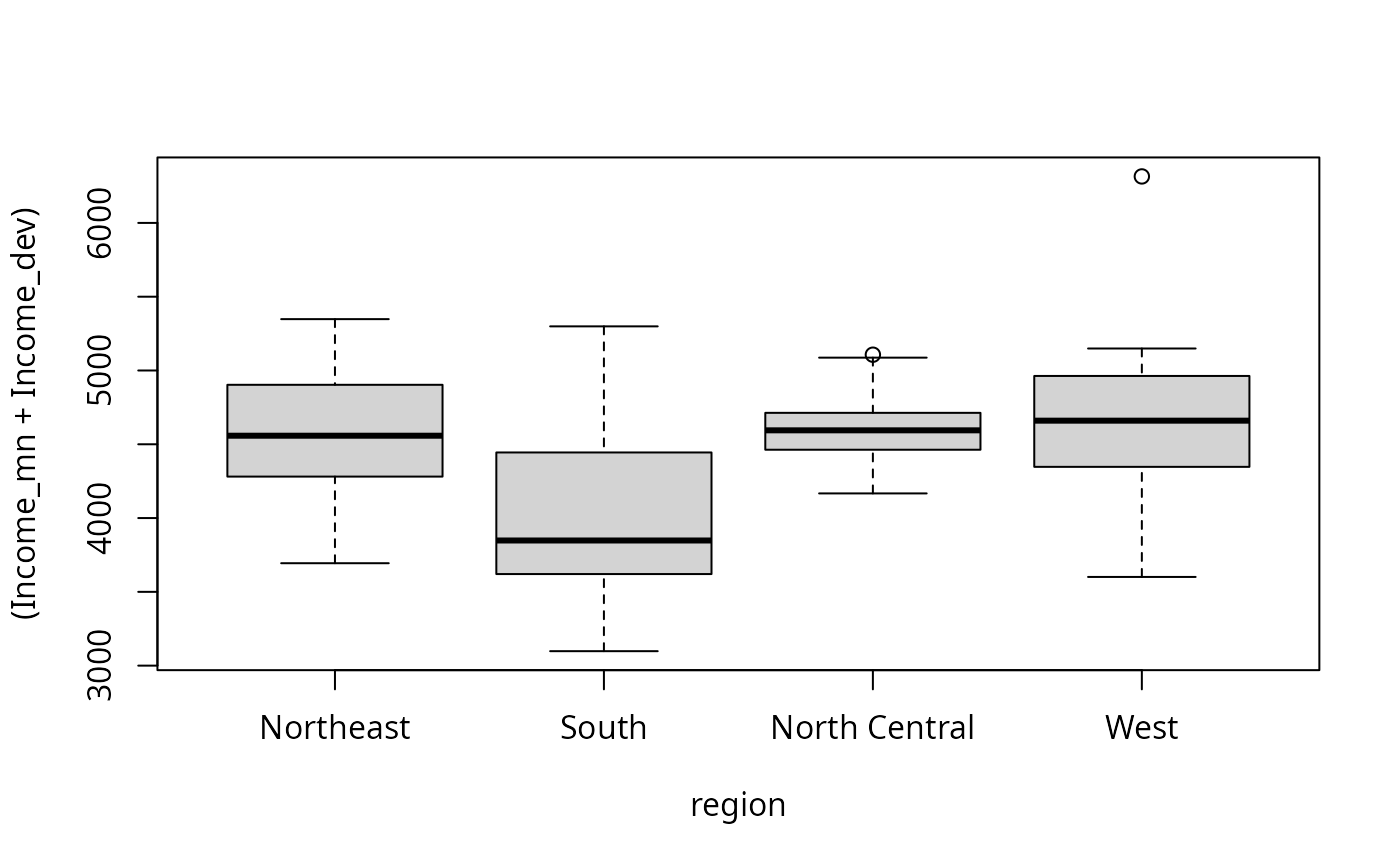
## The following box plots should be identical
boxplot(Income ~ region, statenew.gmc1)
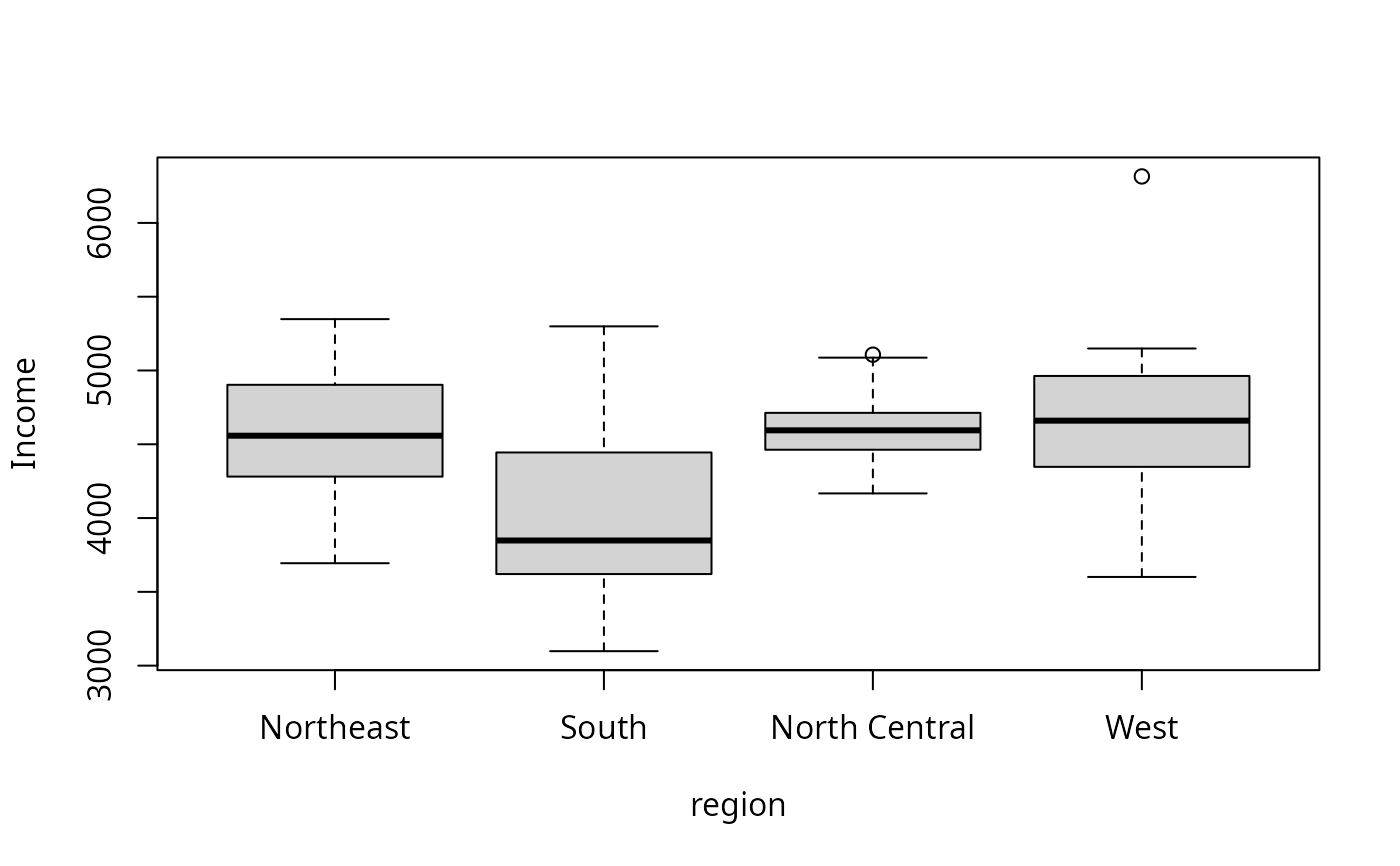 boxplot((Income_mn + Income_dev) ~ region, statenew.gmc1)
 ## Multiple by variables
fakedat <- data.frame(i = 1:200, j = gl(4, 50), k = gl(20, 10),
y1 = rnorm(200), y2 = rnorm(200))
head(gmc(fakedat, "y1", by = "k"), 20)
#> k i j y1 y2 y1_mn y1_dev
#> 1 1 1 1 1.37336867 0.33237530 0.3491879 1.024180779
#> 2 1 2 1 0.47872676 -0.75671192 0.3491879 0.129538867
#> 3 1 3 1 0.04600165 -0.78570952 0.3491879 -0.303186246
#> 4 1 4 1 0.99503577 -0.36386952 0.3491879 0.645847872
#> 5 1 5 1 0.43299958 -0.24836108 0.3491879 0.083811688
#> 6 1 6 1 -0.58830791 1.57152248 0.3491879 -0.937495800
#> 7 1 7 1 -0.38027449 1.21669981 0.3491879 -0.729462380
#> 8 1 8 1 0.53622975 0.26455968 0.3491879 0.187041852
#> 9 1 9 1 -0.90491402 0.31140073 0.3491879 -1.254101918
#> 10 1 10 1 1.50301318 0.74806663 0.3491879 1.153825287
#> 11 2 11 1 2.61648106 0.37560361 0.1026826 2.513798445
#> 12 2 12 1 -0.34045362 -0.19768565 0.1026826 -0.443136241
#> 13 2 13 1 -0.48740245 0.05350647 0.1026826 -0.590085068
#> 14 2 14 1 0.84510827 -0.11894299 0.1026826 0.742425653
#> 15 2 15 1 -1.06618917 -0.06309957 0.1026826 -1.168871785
#> 16 2 16 1 -1.12346914 -0.11600003 0.1026826 -1.226151757
#> 17 2 17 1 0.92263391 -0.19159033 0.1026826 0.819951293
#> 18 2 18 1 -0.30904687 -0.61663967 0.1026826 -0.411729488
#> 19 2 19 1 -0.13712282 1.04284547 0.1026826 -0.239805442
#> 20 2 20 1 0.10628701 -1.43784499 0.1026826 0.003604389
head(gmc(fakedat, "y1", by = c("j", "k"), fulldataframe = FALSE), 40)
#> j k y1_mn y1_dev
#> 1 1 1 0.3491879 1.024180779
#> 2 1 1 0.3491879 0.129538867
#> 3 1 1 0.3491879 -0.303186246
#> 4 1 1 0.3491879 0.645847872
#> 5 1 1 0.3491879 0.083811688
#> 6 1 1 0.3491879 -0.937495800
#> 7 1 1 0.3491879 -0.729462380
#> 8 1 1 0.3491879 0.187041852
#> 9 1 1 0.3491879 -1.254101918
#> 10 1 1 0.3491879 1.153825287
#> 11 1 2 0.1026826 2.513798445
#> 12 1 2 0.1026826 -0.443136241
#> 13 1 2 0.1026826 -0.590085068
#> 14 1 2 0.1026826 0.742425653
#> 15 1 2 0.1026826 -1.168871785
#> 16 1 2 0.1026826 -1.226151757
#> 17 1 2 0.1026826 0.819951293
#> 18 1 2 0.1026826 -0.411729488
#> 19 1 2 0.1026826 -0.239805442
#> 20 1 2 0.1026826 0.003604389
#> 21 1 3 0.2158531 0.724099655
#> 22 1 3 0.2158531 0.538460720
#> 23 1 3 0.2158531 0.579599642
#> 24 1 3 0.2158531 0.534412573
#> 25 1 3 0.2158531 1.232043884
#> 26 1 3 0.2158531 -0.608740671
#> 27 1 3 0.2158531 -1.166064286
#> 28 1 3 0.2158531 -1.768738149
#> 29 1 3 0.2158531 0.639155247
#> 30 1 3 0.2158531 -0.704228616
#> 31 1 4 0.0185566 0.495370692
#> 32 1 4 0.0185566 0.007888569
#> 33 1 4 0.0185566 -1.051561529
#> 34 1 4 0.0185566 -0.837706386
#> 35 1 4 0.0185566 -0.193400259
#> 36 1 4 0.0185566 1.677043800
#> 37 1 4 0.0185566 1.599643268
#> 38 1 4 0.0185566 -0.908735027
#> 39 1 4 0.0185566 -1.096618365
#> 40 1 4 0.0185566 0.308075236
head(gmc(fakedat, c("y1", "y2"), by = c("j", "k"), fulldataframe = FALSE))
#> j k y1_mn y2_mn y1_dev y2_dev
#> 1 1 1 0.3491879 0.2289973 1.02418078 0.1033780
#> 2 1 1 0.3491879 0.2289973 0.12953887 -0.9857092
#> 3 1 1 0.3491879 0.2289973 -0.30318625 -1.0147068
#> 4 1 1 0.3491879 0.2289973 0.64584787 -0.5928668
#> 5 1 1 0.3491879 0.2289973 0.08381169 -0.4773583
#> 6 1 1 0.3491879 0.2289973 -0.93749580 1.3425252
## Check missing value management
fakedat[2, "k"] <- NA
fakedat[4, "j"] <- NA##' head(gmc(fakedat, "y1", by = "k"), 20)
head(gmc(fakedat, "y1", by = c("j", "k"), fulldataframe = FALSE), 40)
#> j k y1_mn y1_dev
#> 1 1 1 0.2522646 1.121104121
#> 2 1 <NA> NA NA
#> 3 1 1 0.2522646 -0.206262904
#> 4 <NA> 1 NA NA
#> 5 1 1 0.2522646 0.180735030
#> 6 1 1 0.2522646 -0.840572458
#> 7 1 1 0.2522646 -0.632539038
#> 8 1 1 0.2522646 0.283965195
#> 9 1 1 0.2522646 -1.157178576
#> 10 1 1 0.2522646 1.250748629
#> 11 1 2 0.1026826 2.513798445
#> 12 1 2 0.1026826 -0.443136241
#> 13 1 2 0.1026826 -0.590085068
#> 14 1 2 0.1026826 0.742425653
#> 15 1 2 0.1026826 -1.168871785
#> 16 1 2 0.1026826 -1.226151757
#> 17 1 2 0.1026826 0.819951293
#> 18 1 2 0.1026826 -0.411729488
#> 19 1 2 0.1026826 -0.239805442
#> 20 1 2 0.1026826 0.003604389
#> 21 1 3 0.2158531 0.724099655
#> 22 1 3 0.2158531 0.538460720
#> 23 1 3 0.2158531 0.579599642
#> 24 1 3 0.2158531 0.534412573
#> 25 1 3 0.2158531 1.232043884
#> 26 1 3 0.2158531 -0.608740671
#> 27 1 3 0.2158531 -1.166064286
#> 28 1 3 0.2158531 -1.768738149
#> 29 1 3 0.2158531 0.639155247
#> 30 1 3 0.2158531 -0.704228616
#> 31 1 4 0.0185566 0.495370692
#> 32 1 4 0.0185566 0.007888569
#> 33 1 4 0.0185566 -1.051561529
#> 34 1 4 0.0185566 -0.837706386
#> 35 1 4 0.0185566 -0.193400259
#> 36 1 4 0.0185566 1.677043800
#> 37 1 4 0.0185566 1.599643268
#> 38 1 4 0.0185566 -0.908735027
#> 39 1 4 0.0185566 -1.096618365
#> 40 1 4 0.0185566 0.308075236
## Multiple by variables
fakedat <- data.frame(i = 1:200, j = gl(4, 50), k = gl(20, 10),
y1 = rnorm(200), y2 = rnorm(200))
head(gmc(fakedat, "y1", by = "k"), 20)
#> k i j y1 y2 y1_mn y1_dev
#> 1 1 1 1 1.37336867 0.33237530 0.3491879 1.024180779
#> 2 1 2 1 0.47872676 -0.75671192 0.3491879 0.129538867
#> 3 1 3 1 0.04600165 -0.78570952 0.3491879 -0.303186246
#> 4 1 4 1 0.99503577 -0.36386952 0.3491879 0.645847872
#> 5 1 5 1 0.43299958 -0.24836108 0.3491879 0.083811688
#> 6 1 6 1 -0.58830791 1.57152248 0.3491879 -0.937495800
#> 7 1 7 1 -0.38027449 1.21669981 0.3491879 -0.729462380
#> 8 1 8 1 0.53622975 0.26455968 0.3491879 0.187041852
#> 9 1 9 1 -0.90491402 0.31140073 0.3491879 -1.254101918
#> 10 1 10 1 1.50301318 0.74806663 0.3491879 1.153825287
#> 11 2 11 1 2.61648106 0.37560361 0.1026826 2.513798445
#> 12 2 12 1 -0.34045362 -0.19768565 0.1026826 -0.443136241
#> 13 2 13 1 -0.48740245 0.05350647 0.1026826 -0.590085068
#> 14 2 14 1 0.84510827 -0.11894299 0.1026826 0.742425653
#> 15 2 15 1 -1.06618917 -0.06309957 0.1026826 -1.168871785
#> 16 2 16 1 -1.12346914 -0.11600003 0.1026826 -1.226151757
#> 17 2 17 1 0.92263391 -0.19159033 0.1026826 0.819951293
#> 18 2 18 1 -0.30904687 -0.61663967 0.1026826 -0.411729488
#> 19 2 19 1 -0.13712282 1.04284547 0.1026826 -0.239805442
#> 20 2 20 1 0.10628701 -1.43784499 0.1026826 0.003604389
head(gmc(fakedat, "y1", by = c("j", "k"), fulldataframe = FALSE), 40)
#> j k y1_mn y1_dev
#> 1 1 1 0.3491879 1.024180779
#> 2 1 1 0.3491879 0.129538867
#> 3 1 1 0.3491879 -0.303186246
#> 4 1 1 0.3491879 0.645847872
#> 5 1 1 0.3491879 0.083811688
#> 6 1 1 0.3491879 -0.937495800
#> 7 1 1 0.3491879 -0.729462380
#> 8 1 1 0.3491879 0.187041852
#> 9 1 1 0.3491879 -1.254101918
#> 10 1 1 0.3491879 1.153825287
#> 11 1 2 0.1026826 2.513798445
#> 12 1 2 0.1026826 -0.443136241
#> 13 1 2 0.1026826 -0.590085068
#> 14 1 2 0.1026826 0.742425653
#> 15 1 2 0.1026826 -1.168871785
#> 16 1 2 0.1026826 -1.226151757
#> 17 1 2 0.1026826 0.819951293
#> 18 1 2 0.1026826 -0.411729488
#> 19 1 2 0.1026826 -0.239805442
#> 20 1 2 0.1026826 0.003604389
#> 21 1 3 0.2158531 0.724099655
#> 22 1 3 0.2158531 0.538460720
#> 23 1 3 0.2158531 0.579599642
#> 24 1 3 0.2158531 0.534412573
#> 25 1 3 0.2158531 1.232043884
#> 26 1 3 0.2158531 -0.608740671
#> 27 1 3 0.2158531 -1.166064286
#> 28 1 3 0.2158531 -1.768738149
#> 29 1 3 0.2158531 0.639155247
#> 30 1 3 0.2158531 -0.704228616
#> 31 1 4 0.0185566 0.495370692
#> 32 1 4 0.0185566 0.007888569
#> 33 1 4 0.0185566 -1.051561529
#> 34 1 4 0.0185566 -0.837706386
#> 35 1 4 0.0185566 -0.193400259
#> 36 1 4 0.0185566 1.677043800
#> 37 1 4 0.0185566 1.599643268
#> 38 1 4 0.0185566 -0.908735027
#> 39 1 4 0.0185566 -1.096618365
#> 40 1 4 0.0185566 0.308075236
head(gmc(fakedat, c("y1", "y2"), by = c("j", "k"), fulldataframe = FALSE))
#> j k y1_mn y2_mn y1_dev y2_dev
#> 1 1 1 0.3491879 0.2289973 1.02418078 0.1033780
#> 2 1 1 0.3491879 0.2289973 0.12953887 -0.9857092
#> 3 1 1 0.3491879 0.2289973 -0.30318625 -1.0147068
#> 4 1 1 0.3491879 0.2289973 0.64584787 -0.5928668
#> 5 1 1 0.3491879 0.2289973 0.08381169 -0.4773583
#> 6 1 1 0.3491879 0.2289973 -0.93749580 1.3425252
## Check missing value management
fakedat[2, "k"] <- NA
fakedat[4, "j"] <- NA##' head(gmc(fakedat, "y1", by = "k"), 20)
head(gmc(fakedat, "y1", by = c("j", "k"), fulldataframe = FALSE), 40)
#> j k y1_mn y1_dev
#> 1 1 1 0.2522646 1.121104121
#> 2 1 <NA> NA NA
#> 3 1 1 0.2522646 -0.206262904
#> 4 <NA> 1 NA NA
#> 5 1 1 0.2522646 0.180735030
#> 6 1 1 0.2522646 -0.840572458
#> 7 1 1 0.2522646 -0.632539038
#> 8 1 1 0.2522646 0.283965195
#> 9 1 1 0.2522646 -1.157178576
#> 10 1 1 0.2522646 1.250748629
#> 11 1 2 0.1026826 2.513798445
#> 12 1 2 0.1026826 -0.443136241
#> 13 1 2 0.1026826 -0.590085068
#> 14 1 2 0.1026826 0.742425653
#> 15 1 2 0.1026826 -1.168871785
#> 16 1 2 0.1026826 -1.226151757
#> 17 1 2 0.1026826 0.819951293
#> 18 1 2 0.1026826 -0.411729488
#> 19 1 2 0.1026826 -0.239805442
#> 20 1 2 0.1026826 0.003604389
#> 21 1 3 0.2158531 0.724099655
#> 22 1 3 0.2158531 0.538460720
#> 23 1 3 0.2158531 0.579599642
#> 24 1 3 0.2158531 0.534412573
#> 25 1 3 0.2158531 1.232043884
#> 26 1 3 0.2158531 -0.608740671
#> 27 1 3 0.2158531 -1.166064286
#> 28 1 3 0.2158531 -1.768738149
#> 29 1 3 0.2158531 0.639155247
#> 30 1 3 0.2158531 -0.704228616
#> 31 1 4 0.0185566 0.495370692
#> 32 1 4 0.0185566 0.007888569
#> 33 1 4 0.0185566 -1.051561529
#> 34 1 4 0.0185566 -0.837706386
#> 35 1 4 0.0185566 -0.193400259
#> 36 1 4 0.0185566 1.677043800
#> 37 1 4 0.0185566 1.599643268
#> 38 1 4 0.0185566 -0.908735027
#> 39 1 4 0.0185566 -1.096618365
#> 40 1 4 0.0185566 0.308075236