Create an ordinal variable by grouping numeric data input.
cutFancy.RdThis is a convenience function for usage of R's cut
function. Users can specify cutpoints or category labels or
desired proportions of groups in various ways. In that way, it has
a more flexible interface than cut. It also tries to notice
and correct some common user errors, such as omitting the outer
boundaries from the probs argument. The returned values are
labeled by their midpoints, rather than cut's usual boundaries.
Arguments
- y
The input data from which the categorized variable will be created.
- cutpoints
Optional paramter, a vector of thresholds at which to cut the data. If it is not supplied, the default value
cutpoints="quantile"will take effect. Users can supplement withprobsand/orcategoriesas shown in examples.- probs
This is an optional parameter, relevant only when the R function
quantilefunction is used to calculate cutpoints. The length should be number of desired categories PLUS ONE, as inc(0, .3, .6, 1). That will create categories that represent 1) less than .3, between .3 and .6, and above .6. A common user error is to specify only the internal divider values, such asprobs = c(.3, .6). To anticipate and correct that error, this function will insert the lower limit of 0 and the upper limit of 1 if they are not already present inprobs.- categories
Can be a number to designate the number of sub-groups created, or it can be a vector of names used. If
cutpointsandprobsare not specified, the parametercategoriesshould be an integer to specify how many data groups to create.It is required if cutpoints="quantile" and probs is not specified. Can also be a vector of names to be used for the categories that are created. If category names are not provided, the names for the ordinal variable will be the midpoint of the numeric range from which they are constructed.
Details
The dividing points, thought of as "thresholds" or "cutpoints",
can be specified in several ways. cutFancy will
automatically create equally-sized sets of observations for a
given number of categories if neither probs nor
cutpoints is specified. The bare minimum input needed is
categories=5, for example, to ask for 5 equally sized
groups. More user control can be had by specifying either
cutpoints or probs. If cutpoints is not
specified at all, or if cutpoints="quantile", then
probs can be used to specify the proportions of the data
points that are to fall within each range. On the other hand, one
can specify cutpoints = "quantile" and then probs will
be used to specify the proportions of the data points that are to
fall within each range.
If categories is not specified, the category names will be
created. Names for ordinal categories will be the numerical
midpoints for the outcomes. Perhaps this will deviate from your
expectation, which might be ordinal categories name "0", "1", "2",
and so forth. The numerically labeled values we provide can be
used in various ways during the analysis process. Read "?factor"
to learn ways to convert the ordinal output to other
formats. Examples include various ways of converting the ordinal
output to numeric.
The categories parameter works together with
cutpoints. cutpoints allows a character string
"quantile". If cutpoints is not specified, or if the user
specifies a character string cutpoints="quantile", then the
probs would be used to determine the cutpoints. However,
if probs is not specified, then the categories
argument can be used. If cutpoints="quantile", then
if
categoriesis one integer, then it is interpreted as the number of "equally sized" categories to be created, orcategoriescan be a vector of names. The length of the vector is used to determine the number of categories, and the values are put to use as factor labels.
Examples
set.seed(234234)
y <- rnorm(1000, m = 35, sd = 14)
yord <- cutFancy(y, cutpoints = c(30, 40, 50))
table(yord)
#> yord
#> 11 35 45 69
#> 343 302 209 146
attr(yord, "props")
#> yord
#> 11 35 45 69
#> 0.343 0.302 0.209 0.146
attr(yord, "cutpoints")
#> [1] 30 40 50
yord <- cutFancy(y, categories = 4L)
table(yord, exclude = NULL)
#> yord
#> 9.5 31 40 66
#> 250 250 250 250
attr(yord, "props")
#> yord
#> 9.5 31 40 66
#> 0.25 0.25 0.25 0.25
attr(yord, "cutpoints")
#> [1] 26.17132 35.13526 44.83495
yord <- cutFancy(y, probs = c(0, .1, .3, .7, .9, 1.0),
categories = c("A", "B", "C", "D", "E"))
table(yord, exclude = NULL)
#> yord
#> A B C D E
#> 100 200 400 200 100
attr(yord, "props")
#> yord
#> A B C D E
#> 0.1 0.2 0.4 0.2 0.1
attr(yord, "cutpoints")
#> [1] 17.44649 27.99351 42.01381 53.10705
yord <- cutFancy(y, probs = c(0, .1, .3, .7, .9, 1.0))
table(yord, exclude = NULL)
#> yord
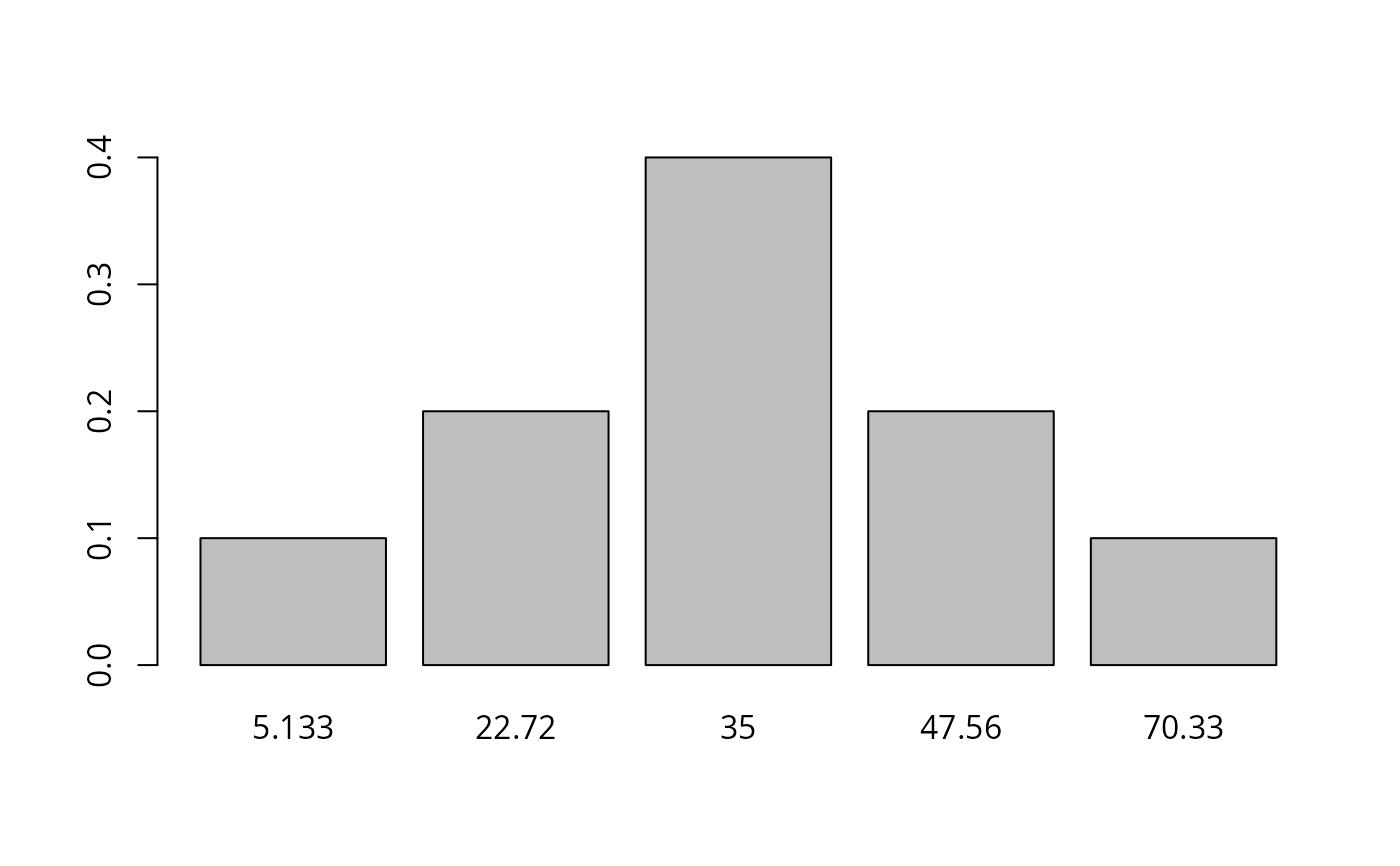
#> 5.133 22.72 35 47.56 70.33
#> 100 200 400 200 100
attr(yord, "props")
#> yord
#> 5.133 22.72 35 47.56 70.33
#> 0.1 0.2 0.4 0.2 0.1
attr(yord, "cutpoints")
#> [1] 17.44649 27.99351 42.01381 53.10705
yasinteger <- as.integer(yord)
table(yasinteger, yord)
#> yord
#> yasinteger 5.133 22.72 35 47.56 70.33
#> 1 100 0 0 0 0
#> 2 0 200 0 0 0
#> 3 0 0 400 0 0
#> 4 0 0 0 200 0
#> 5 0 0 0 0 100
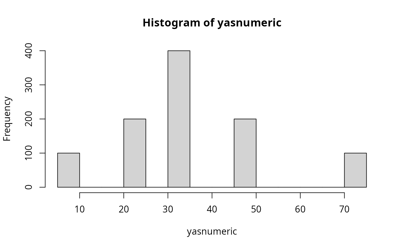
yasnumeric <- as.numeric(levels(yord))[yord]
table(yasnumeric, yord)
#> yord
#> yasnumeric 5.133 22.72 35 47.56 70.33
#> 5.133 100 0 0 0 0
#> 22.72 0 200 0 0 0
#> 35 0 0 400 0 0
#> 47.56 0 0 0 200 0
#> 70.33 0 0 0 0 100
barplot(attr(yord, "props"))
 hist(yasnumeric)
 X1a <-
genCorrelatedData3("y ~ 1.1 + 2.1 * x1 + 3 * x2 + 3.5 * x3 + 1.1 * x1:x3",
N = 10000, means = c(x1 = 1, x2 = -1, x3 = 3),
sds = 1, rho = 0.4)
## Create cutpoints from quantiles
probs <- c(.3, .6)
X1a$yord <- cutFancy(X1a$y, probs = probs)
attributes(X1a$yord)
#> $levels
#> [1] "-3.639" "12.48" "40.58"
#>
#> $class
#> [1] "ordered" "factor"
#>
#> $cutpoints
#> [1] 8.527858 16.424791
#>
#> $props
#> yord
#> -3.639 12.48 40.58
#> 0.3 0.3 0.4
#>
table(X1a$yord, exclude = NULL)
#>
#> -3.639 12.48 40.58
#> 3000 3000 4000
X1a <-
genCorrelatedData3("y ~ 1.1 + 2.1 * x1 + 3 * x2 + 3.5 * x3 + 1.1 * x1:x3",
N = 10000, means = c(x1 = 1, x2 = -1, x3 = 3),
sds = 1, rho = 0.4)
## Create cutpoints from quantiles
probs <- c(.3, .6)
X1a$yord <- cutFancy(X1a$y, probs = probs)
attributes(X1a$yord)
#> $levels
#> [1] "-3.639" "12.48" "40.58"
#>
#> $class
#> [1] "ordered" "factor"
#>
#> $cutpoints
#> [1] 8.527858 16.424791
#>
#> $props
#> yord
#> -3.639 12.48 40.58
#> 0.3 0.3 0.4
#>
table(X1a$yord, exclude = NULL)
#>
#> -3.639 12.48 40.58
#> 3000 3000 4000