Robust Covariance Matrix Estimates

Uses the Huber-White method to adjust the variance-covariance matrix of a fit from maximum likelihood or least squares, to correct for heteroscedasticity and for correlated responses from cluster samples. The method uses the ordinary estimates of regression coefficients and other parameters of the model, but involves correcting the covariance matrix for model misspecification and sampling design. Models currently implemented are models that have a residuals(fit,type="score") function implemented, such as lrm, cph, coxph, and ordinary linear models (ols). The fit must have specified the x=TRUE and y=TRUE options for certain models. Observations in different clusters are assumed to be independent. For the special case where every cluster contains one observation, the corrected covariance matrix returned is the "sandwich" estimator (see Lin and Wei). This is a consistent estimate of the covariance matrix even if the model is misspecified (e.g. heteroscedasticity, underdispersion, wrong covariate form).

For the special case of ols fits, robcov can compute the improved (especially for small samples) Efron estimator that adjusts for natural heterogeneity of residuals (see Long and Ervin (2000) estimator HC3).

Usage

robcov(fit, cluster, method=c('huber','efron'))

Arguments

fit: a fit object from the rms series
cluster: a variable indicating groupings. cluster may be any type of vector (factor, character, integer). NAs are not allowed. Unique values of cluster indicate possibly correlated groupings of observations. Note the data used in the fit and stored in fit$x and fit$y may have had observations containing missing values deleted. It is assumed that if any NAs were removed during the original model fitting, an naresid function exists to restore NAs so that the rows of the score matrix coincide with cluster. If cluster is omitted, it defaults to the integers 1,2,...,n to obtain the "sandwich" robust covariance matrix estimate.
method: can set to "efron" for ols fits (only). Default is Huber-White estimator of the covariance matrix.

Value

a new fit object with the same class as the original fit, and with the element orig.var added. orig.var is the covariance matrix of the original fit. Also, the original var component is replaced with the new Huberized estimates. A component clusterInfo is added to contain elements name and n holding the name of the cluster variable and the number of clusters.

Author

Frank Harrell
Department of Biostatistics
Vanderbilt University
fh@fharrell.com

References

Huber, PJ. Proc Fifth Berkeley Symposium Math Stat 1:221–33, 1967.

White, H. Econometrica 50:1–25, 1982.

Lin, DY, Wei, LJ. JASA 84:1074–8, 1989.

Rogers, W. Stata Technical Bulletin STB-8, p. 15–17, 1992.

Rogers, W. Stata Release 3 Manual, deff, loneway, huber, hreg, hlogit functions.

Long, JS, Ervin, LH. The American Statistician 54:217–224, 2000.

Examples

# In OLS test against more manual approach
set.seed(1)
n <- 15
x1 <- 1:n
x2 <- sample(1:n)
y <- round(x1 + x2 + 8*rnorm(n))
f <- ols(y ~ x1 + x2, x=TRUE, y=TRUE)
vcov(f)
#>           Intercept        x1        x2
#> Intercept   23.1202 -1.217386 -1.217386
#> x1          -1.2174  0.211983 -0.059809
#> x2          -1.2174 -0.059809  0.211983
vcov(robcov(f))
#>           Intercept        x1        x2
#> Intercept  29.74046 -1.934103 -0.969979
#> x1         -1.93410  0.205674 -0.010337
#> x2         -0.96998 -0.010337  0.121852
X <- f$x
G <- diag(resid(f)^2)
solve(t(X) %*% X) %*% (t(X) %*% G %*% X) %*% solve(t(X) %*% X)
#>           x1        x2
#> x1  0.084451 -0.080795
#> x2 -0.080795  0.102160

# Duplicate data and adjust for intra-cluster correlation to see that
# the cluster sandwich estimator completely ignored the duplicates
x1 <- c(x1,x1)
x2 <- c(x2,x2)
y  <- c(y, y)
g <- ols(y ~ x1 + x2, x=TRUE, y=TRUE)
vcov(robcov(g, c(1:n, 1:n)))
#>           Intercept        x1        x2
#> Intercept  29.74046 -1.934103 -0.969979
#> x1         -1.93410  0.205674 -0.010337
#> x2         -0.96998 -0.010337  0.121852

# A dataset contains a variable number of observations per subject,
# and all observations are laid out in separate rows. The responses
# represent whether or not a given segment of the coronary arteries
# is occluded. Segments of arteries may not operate independently
# in the same patient.  We assume a "working independence model" to
# get estimates of the coefficients, i.e., that estimates assuming
# independence are reasonably efficient.  The job is then to get
# unbiased estimates of variances and covariances of these estimates.

n.subjects <- 30
ages <- rnorm(n.subjects, 50, 15)
sexes  <- factor(sample(c('female','male'), n.subjects, TRUE))
logit <- (ages-50)/5
prob <- plogis(logit)  # true prob not related to sex
id <- sample(1:n.subjects, 300, TRUE) # subjects sampled multiple times
table(table(id))  # frequencies of number of obs/subject
#> 
#>  2  5  6  7  8  9 10 11 12 13 14 15 
#>  1  1  1  2  5  4  2  4  4  1  3  2 
age <- ages[id]
sex <- sexes[id]
# In truth, observations within subject are independent:
y   <- ifelse(runif(300) <= prob[id], 1, 0)
f <- lrm(y ~ lsp(age,50)*sex, x=TRUE, y=TRUE)
g <- robcov(f, id)
diag(g$var)/diag(f$var)
#> <0 x 0 matrix>
# add ,group=w to re-sample from within each level of w
anova(g)            # cluster-adjusted Wald statistics
#>                 Wald Statistics          Response: y 
#> 
#>  Factor                                   Chi-Square d.f. P     
#>  age  (Factor+Higher Order Factors)       107.90     4    <.0001
#>   All Interactions                          1.42     2    0.4924
#>   Nonlinear (Factor+Higher Order Factors)   2.57     2    0.2770
#>  sex  (Factor+Higher Order Factors)         2.01     3    0.5707
#>   All Interactions                          1.42     2    0.4924
#>  age * sex  (Factor+Higher Order Factors)   1.42     2    0.4924
#>   Nonlinear                                 0.65     1    0.4210
#>   Nonlinear Interaction : f(A,B) vs. AB     0.65     1    0.4210
#>  TOTAL NONLINEAR                            2.57     2    0.2770
#>  TOTAL NONLINEAR + INTERACTION              3.33     3    0.3435
#>  TOTAL                                    110.08     5    <.0001
# fastbw(g)         # cluster-adjusted backward elimination
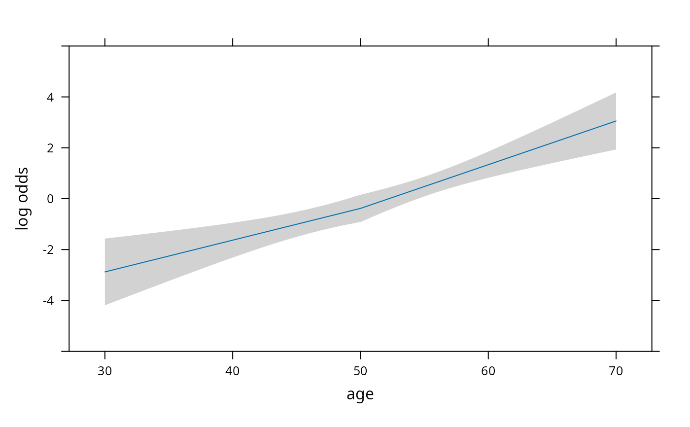
plot(Predict(g, age=30:70, sex='female'))  # cluster-adjusted confidence bands

# or use ggplot(...)

# Get design effects based on inflation of the variances when compared
# with bootstrap estimates which ignore clustering
g2 <- robcov(f)
diag(g$var)/diag(g2$var)
#>       Intercept             age            age'        sex=male  age * sex=male 
#>         0.67183         0.59597         0.53733         0.89149         0.88099 
#> age' * sex=male 
#>         0.93219 


# Get design effects based on pooled tests of factors in model
anova(g2)[,1] / anova(g)[,1]
#>       age  (Factor+Higher Order Factors) 
#>                                  0.86843 
#>                         All Interactions 
#>                                  0.92569 
#>  Nonlinear (Factor+Higher Order Factors) 
#>                                  1.08275 
#>       sex  (Factor+Higher Order Factors) 
#>                                  0.68018 
#>                         All Interactions 
#>                                  0.92569 
#> age * sex  (Factor+Higher Order Factors) 
#>                                  0.92569 
#>                                Nonlinear 
#>                                  0.93219 
#>    Nonlinear Interaction : f(A,B) vs. AB 
#>                                  0.93219 
#>                          TOTAL NONLINEAR 
#>                                  1.08275 
#>            TOTAL NONLINEAR + INTERACTION 
#>                                  1.05470 
#>                                    TOTAL 
#>                                  0.85139 




# A dataset contains one observation per subject, but there may be
# heteroscedasticity or other model misspecification. Obtain
# the robust sandwich estimator of the covariance matrix.


# f <- ols(y ~ pol(age,3), x=TRUE, y=TRUE)
# f.adj <- robcov(f)