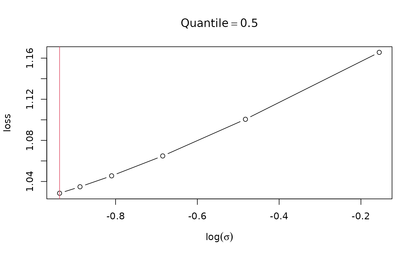
Visual checks for the output of tuneLearnFast()

Provides some visual checks to verify whether the Brent optimizer used by tuneLearnFast() worked correctly.

Usage

# S3 method for class 'learnFast'
check(obj, sel = NULL, ...)

Arguments

obj

the output of a call to tuneLearnFast.

sel

integer vector determining which of the plots will be produced. For instance if sel = c(1, 3) only the 1st and 3rd plots are showed. No entry of sel can be bigger than one plus the number of quantiles considered in the original tuneLearnFast() call. That is, if we estimated the learning rate for qu = c(0.1, 0.4), then max(sel) must be <= 3.

...

currently not used, here only for compatibility reasons.

Value

It produces several plots.

Details

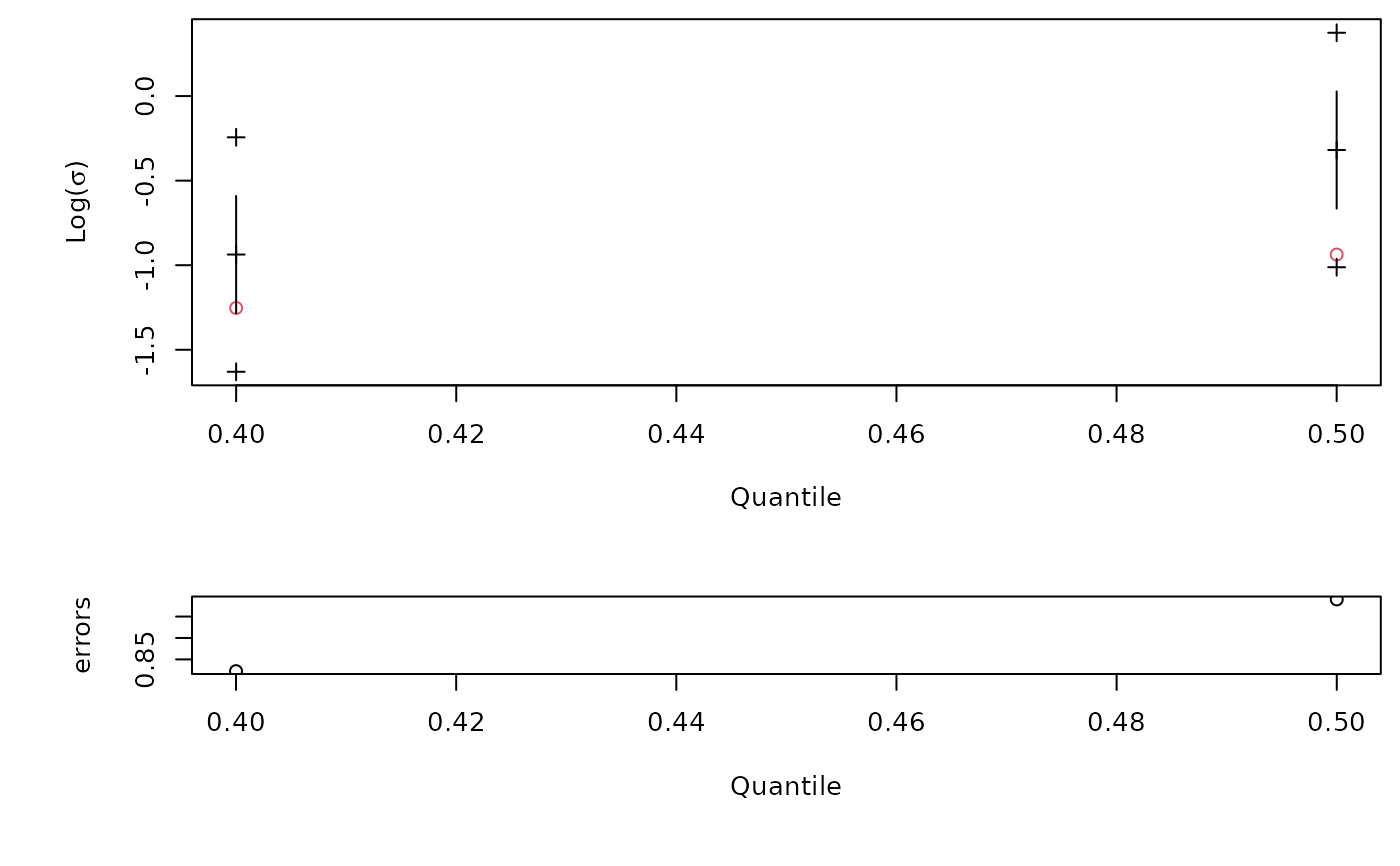
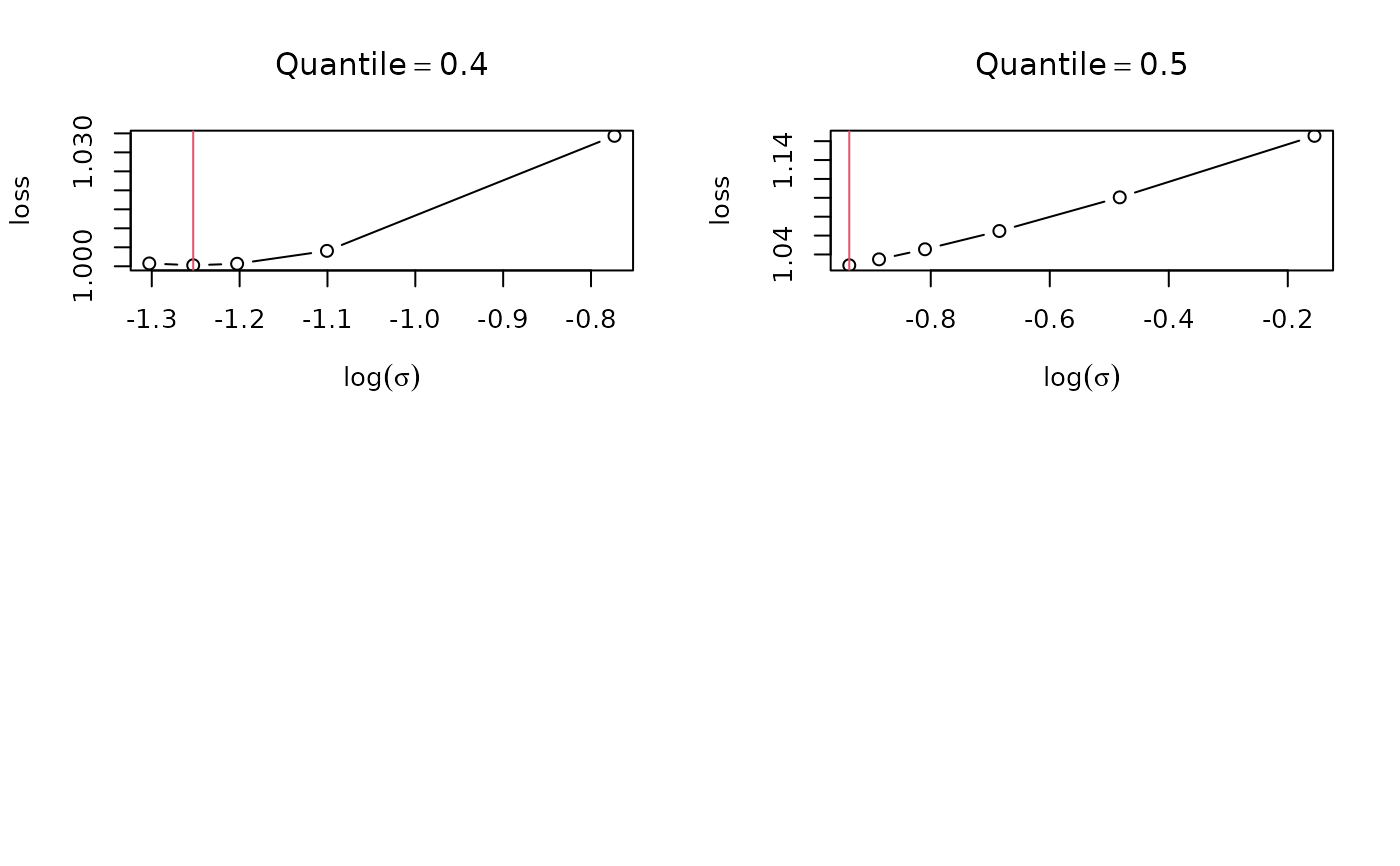
The top plot in the first page shows the bracket used to estimate log(sigma) for each quantile. The brackets are delimited by the crosses and the red dots are the estimates. If a dot falls very close to one of the crosses, that might indicate problems. The bottom plot shows, for each quantile, the value of parameter err used. Sometimes the algorithm needs to increase err above its user-defined value to achieve convergence. Subsequent plots show, for each quantile, the value of the loss function corresponding to each value of log(sigma) explored by Brent algorithm.

References

Fasiolo, M., Wood, S.N., Zaffran, M., Nedellec, R. and Goude, Y., 2020. Fast calibrated additive quantile regression. Journal of the American Statistical Association (to appear). doi:10.1080/01621459.2020.1725521 .

Author

Matteo Fasiolo <matteo.fasiolo@gmail.com>.

Examples

library(qgam)
set.seed(525)
dat <- gamSim(1, n=200)
#> Gu & Wahba 4 term additive model
b <- tuneLearnFast(y ~ s(x0)+s(x1)+s(x2)+s(x3), 
                   data = dat, qu = c(0.4, 0.5), 
                   control = list("tol" = 0.05)) # <- sloppy tolerance to speed-up calibration 
#> Estimating learning rate. Each dot corresponds to a loss evaluation. 
#> qu = 0.5......done 
#> qu = 0.4.....done 
check(b) 


check(b, 3) # Produces only third plot