Convert Cartesian factor loadings into polar coordinates

Factor and cluster analysis output typically presents item by factor correlations (loadings). Tables of factor loadings are frequently sorted by the size of loadings. This style of presentation tends to make it difficult to notice the pattern of loadings on other, secondary, dimensions. By converting to polar coordinates, it is easier to see the pattern of the secondary loadings.

polar(f, sort = TRUE)

Arguments

f

A matrix of loadings or the output from a factor or cluster analysis program

sort

sort=TRUE: sort items by the angle of the items on the first pair of factors.

Details

Although many uses of factor analysis/cluster analysis assume a simple structure where items have one and only one large loading, some domains such as personality or affect items have a more complex structure and some items have high loadings on two factors. (These items are said to have complexity 2, see VSS). By expressing the factor loadings in polar coordinates, this structure is more readily perceived.

For each pair of factors, item loadings are converted to an angle with the first factor, and a vector length corresponding to the amount of variance in the item shared with the two factors.

For a two dimensional structure, this will lead to a column of angles and a column of vector lengths. For n factors, this leads to n* (n-1)/2 columns of angles and an equivalent number of vector lengths.

Value

polar

A data frame of polar coordinates

References

Rafaeli, E. & Revelle, W. (2006). A premature consensus: Are happiness and sadness truly opposite affects? Motivation and Emotion. \

Hofstee, W. K. B., de Raad, B., & Goldberg, L. R. (1992). Integration of the big five and circumplex approaches to trait structure. Journal of Personality and Social Psychology, 63, 146-163.

Author

William Revelle

See also

ICLUST, cluster.plot, circ.tests, fa

Examples

circ.data <- circ.sim(24,500)
circ.fa <- fa(circ.data,2)
circ.polar <- round(polar(circ.fa),2)
circ.polar
#>     Var theta21 vecl21
#> v10  10    4.00   0.57
#> v11  11   14.33   0.60
#> v12  12   27.79   0.62
#> v13  13   36.09   0.59
#> v14  14   59.44   0.66
#> v15  15   74.97   0.61
#> v16  16   87.81   0.59
#> v17  17  106.49   0.63
#> v18  18  109.51   0.59
#> v19  19  137.79   0.63
#> v20  20  149.17   0.60
#> v21  21  169.02   0.62
#> v22  22  181.43   0.61
#> v23  23  202.83   0.57
#> v24  24  208.78   0.57
#> v1    1  216.36   0.54
#> v2    2  239.79   0.58
#> v3    3  252.69   0.63
#> v4    4  268.98   0.60
#> v5    5  285.78   0.59
#> v6    6  301.23   0.56
#> v7    7  317.75   0.58
#> v8    8  331.92   0.58
#> v9    9  341.28   0.62
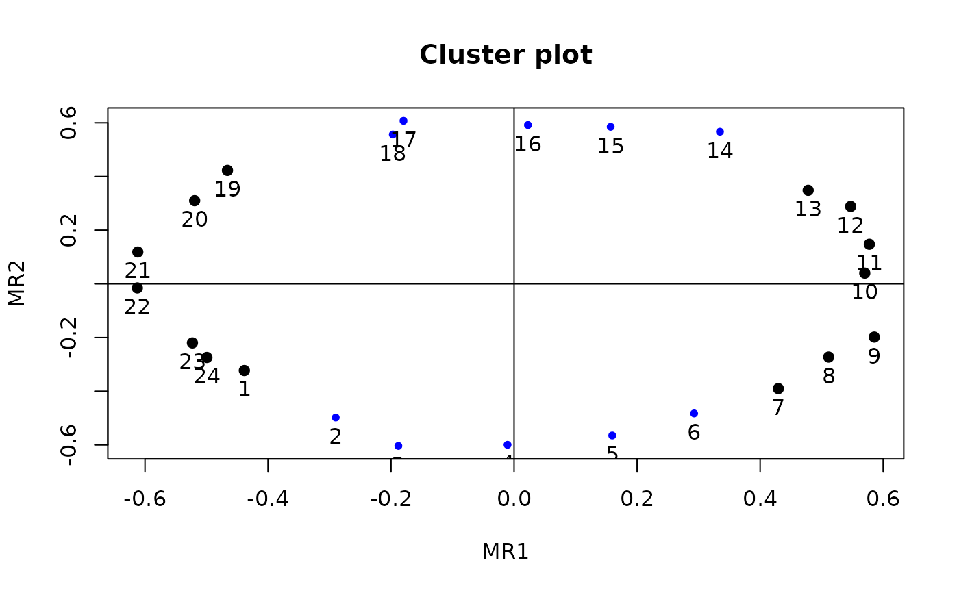
#compare to the graphic
cluster.plot(circ.fa)