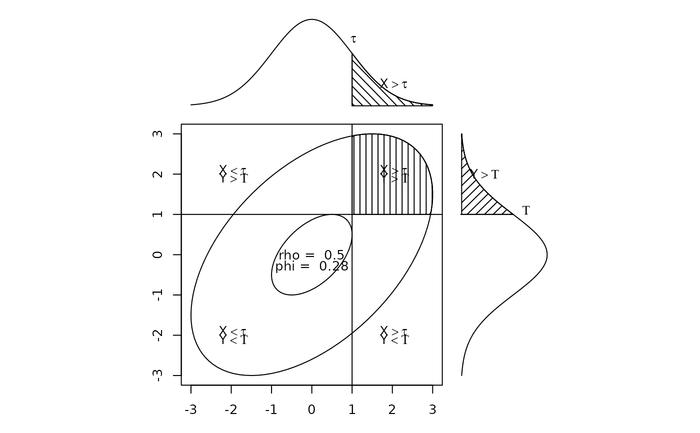
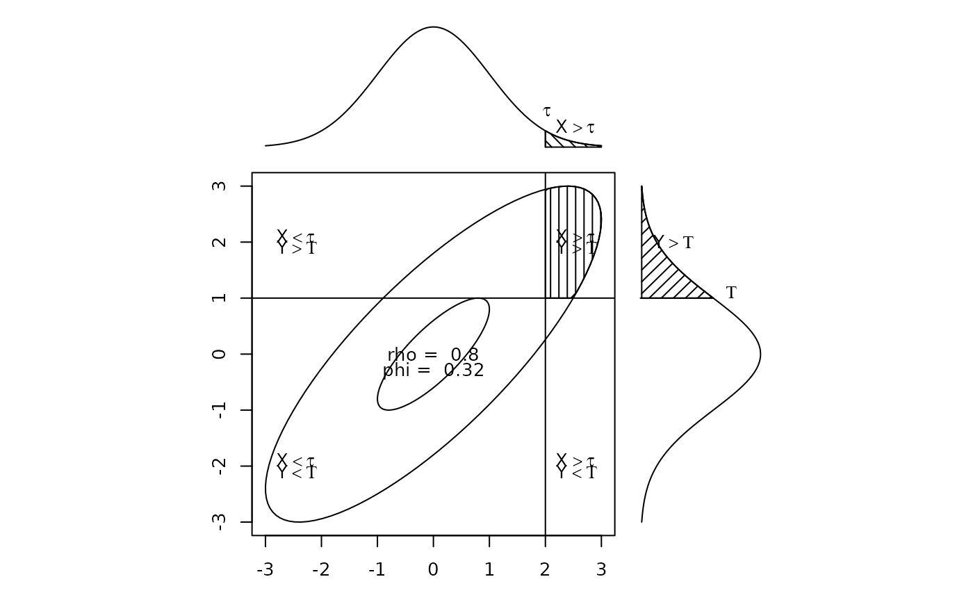
Draw a correlation ellipse and two normal curves to demonstrate tetrachoric correlation
draw.tetra.RdA graphic of a correlation ellipse divided into 4 regions based upon x and y cutpoints on two normal distributions. This is also an example of using the layout function. Draw a bivariate density plot to show how tetrachorics work.
draw.tetra(r, t1, t2,shade=TRUE)
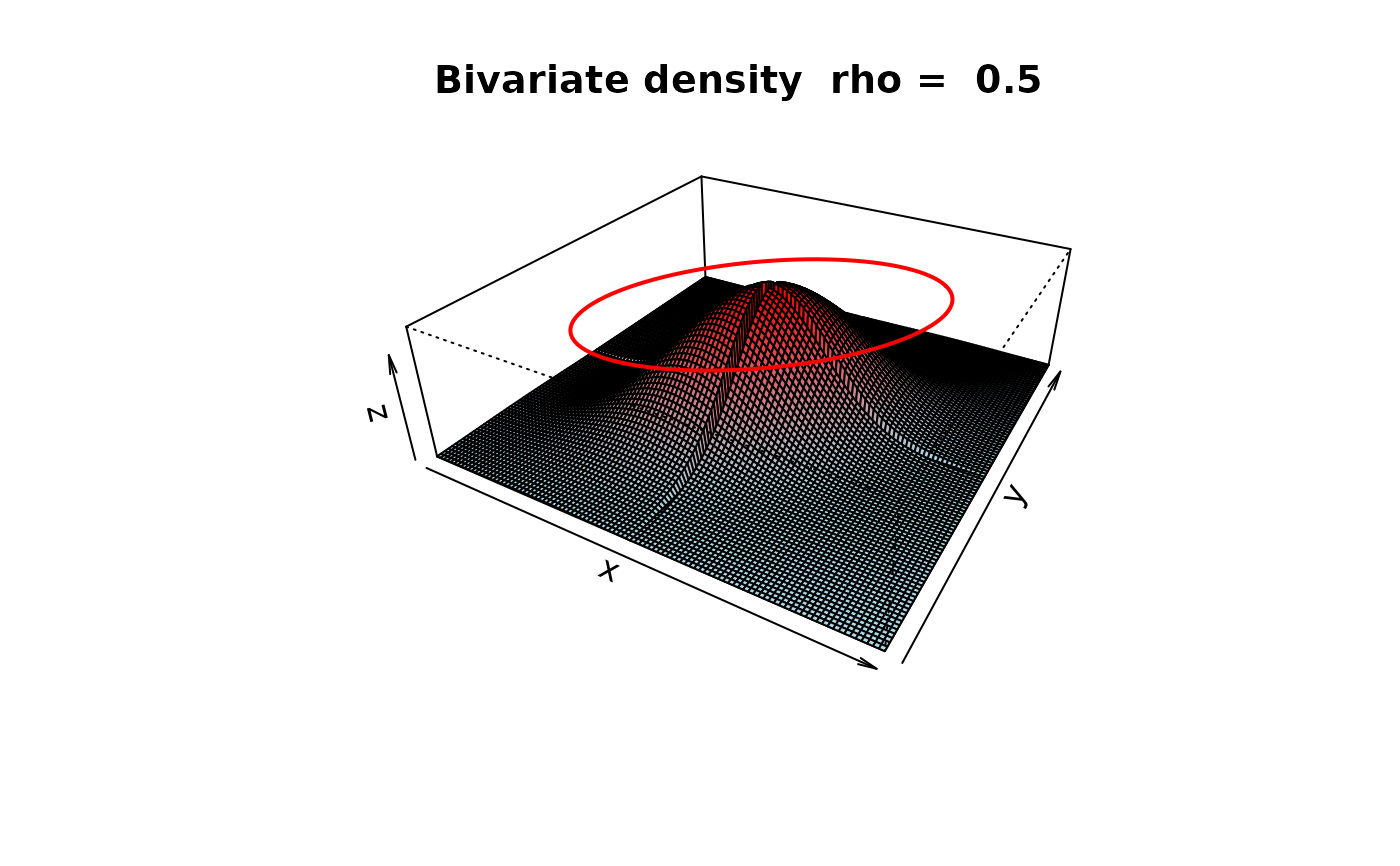
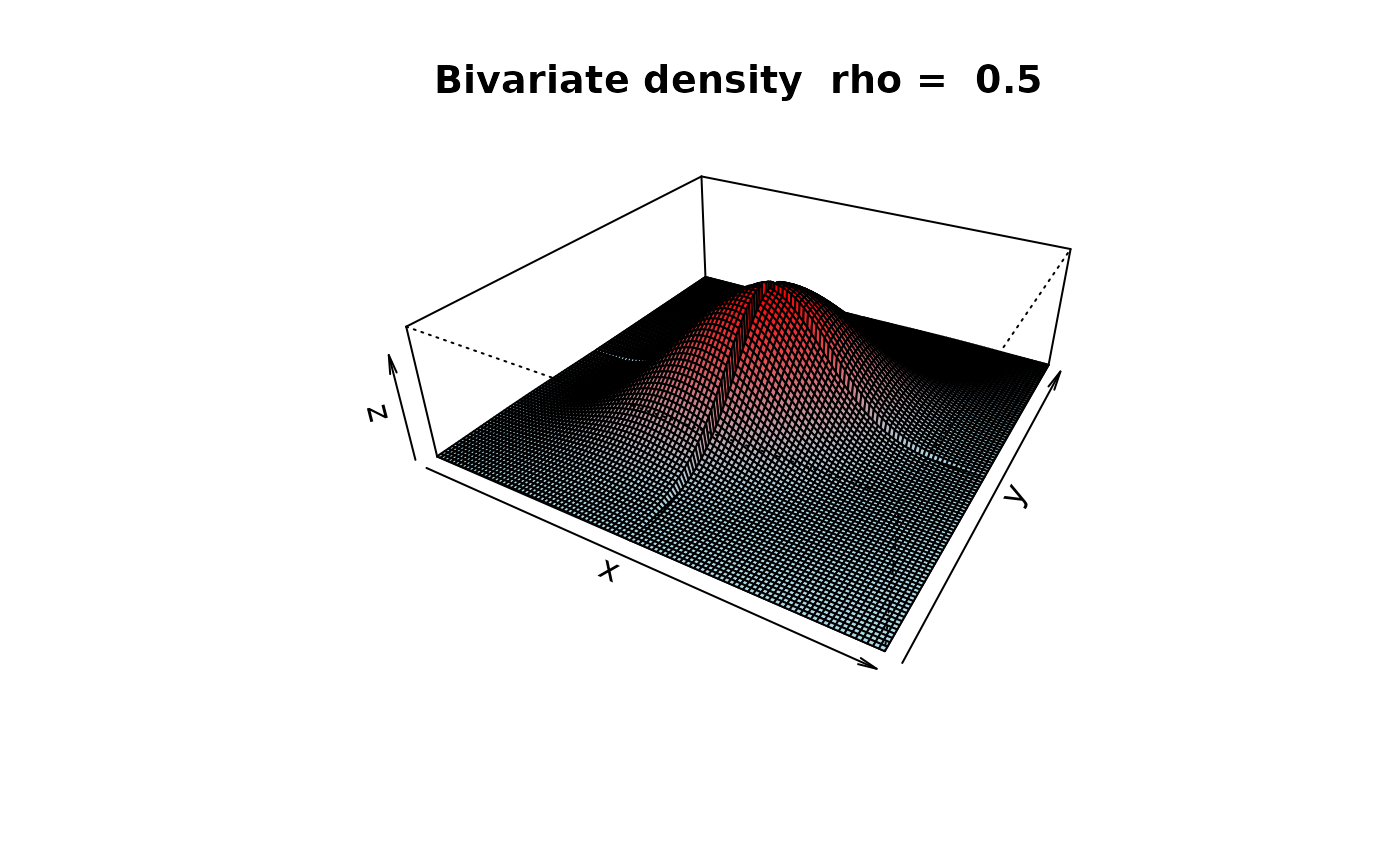
draw.cor(r=.5,expand=10,theta=30,phi=30,N=101,nbcol=30,box=TRUE,
main="Bivariate density rho = ",cuts=NULL,all=TRUE,ellipses=TRUE,ze=.15)Arguments
- r
the underlying Pearson correlation defines the shape of the ellipse
- t1
X is cut at tau
- t2
Y is cut at Tau
- shade
shade the diagram (default is TRUE)
- expand
The relative height of the z axis
- theta
The angle to rotate the x-y plane
- phi
The angle above the plane to view the graph
- N
The grid resolution
- nbcol
The color resolution
- box
Draw the axes
- main
The main title
- cuts
Should the graphic show cuts (e.g., cuts=c(0,0))
- all
Show all four parts of the tetrachoric
- ellipses
Draw a correlation ellipse
- ze
height of the ellipse if requested
Details
A graphic demonstration of the tetrachoric correlation. Used for teaching purposes. The default values are for a correlation of .5 with cuts at 1 and 1. Any other values are possible. The code is also a demonstration of how to use the layout function for complex graphics using base graphics.
See also
tetrachoric to find tetrachoric correlations, irt.fa and fa.poly to use them in factor analyses, scatter.hist to show correlations and histograms.
Examples
#if(require(mvtnorm)) {
#draw.tetra(.5,1,1)
#draw.tetra(.8,2,1)} else {print("draw.tetra requires the mvtnorm package")
#draw.cor(.5,cuts=c(0,0))}

draw.tetra(.5,1,1)

draw.tetra(.8,2,1)

draw.cor(.5,cuts=c(0,0))