9 Cognitive variables discussed by Tucker and Lewis (1973)
Tucker.RdTucker and Lewis (1973) introduced a reliability coefficient for ML factor analysis. Their example data set was previously reported by Tucker (1958) and taken from Thurstone and Thurstone (1941). The correlation matrix is a 9 x 9 for 710 subjects and has two correlated factors of ability: Word Fluency and Verbal.
data(Tucker)Format
A data frame with 9 observations on the following 9 variables.
t42Prefixes
t54Suffixes
t45Chicago Reading Test: Vocabulary
t46Chicago Reading Test: Sentences
t23First and last letters
t24First letters
t27Four letter words
t10Completion
t51Same or Opposite
Details
The correlation matrix from Tucker (1958) was used in Tucker and Lewis (1973) for the Tucker-Lewis Index of factoring reliability.
Source
Tucker, Ledyard (1958) An inter-battery method of factor analysis, Psychometrika, 23, 111-136.
References
L.~Tucker and C.~Lewis. (1973) A reliability coefficient for maximum likelihood factor analysis. Psychometrika, 38(1):1–10.
F.~J. Floyd and K.~F. Widaman. (1995) Factor analysis in the development and refinement of clinical assessment instruments., Psychological Assessment, 7(3):286 – 299.
Examples
data(Tucker)
fa(Tucker,2,n.obs=710)
#> Factor Analysis using method = minres
#> Call: fa(r = Tucker, nfactors = 2, n.obs = 710)
#> Standardized loadings (pattern matrix) based upon correlation matrix
#> MR1 MR2 h2 u2 com
#> t42 -0.04 0.71 0.48 0.52 1.0
#> t54 0.02 0.71 0.51 0.49 1.0
#> t45 0.92 -0.04 0.82 0.18 1.0
#> t46 0.87 -0.06 0.71 0.29 1.0
#> t23 -0.02 0.71 0.50 0.50 1.0
#> t24 0.00 0.74 0.55 0.45 1.0
#> t27 0.11 0.59 0.42 0.58 1.1
#> t10 0.76 0.13 0.68 0.32 1.1
#> t51 0.78 0.05 0.65 0.35 1.0
#>
#> MR1 MR2
#> SS loadings 2.84 2.47
#> Proportion Var 0.32 0.27
#> Cumulative Var 0.32 0.59
#> Proportion Explained 0.54 0.46
#> Cumulative Proportion 0.54 1.00
#>
#> With factor correlations of
#> MR1 MR2
#> MR1 1.00 0.43
#> MR2 0.43 1.00
#>
#> Mean item complexity = 1
#> Test of the hypothesis that 2 factors are sufficient.
#>
#> df null model = 36 with the objective function = 4.49 with Chi Square = 3165.93
#> df of the model are 19 and the objective function was 0.07
#>
#> The root mean square of the residuals (RMSR) is 0.02
#> The df corrected root mean square of the residuals is 0.03
#>
#> The harmonic n.obs is 710 with the empirical chi square 22.23 with prob < 0.27
#> The total n.obs was 710 with Likelihood Chi Square = 50.45 with prob < 0.00011
#>
#> Tucker Lewis Index of factoring reliability = 0.981
#> RMSEA index = 0.048 and the 90 % confidence intervals are 0.032 0.065
#> BIC = -74.29
#> Fit based upon off diagonal values = 1
#> Measures of factor score adequacy
#> MR1 MR2
#> Correlation of (regression) scores with factors 0.96 0.91
#> Multiple R square of scores with factors 0.92 0.84
#> Minimum correlation of possible factor scores 0.83 0.67
omega(Tucker,2)
#>
#> Three factors are required for identification -- general factor loadings set to be equal.
#> Proceed with caution.
#> Think about redoing the analysis with alternative values of the 'option' setting.
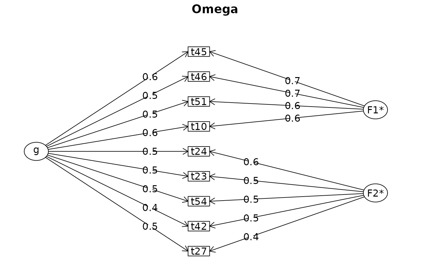 #> Omega
#> Call: omegah(m = m, nfactors = nfactors, fm = fm, key = key, flip = flip,
#> digits = digits, title = title, sl = sl, labels = labels,
#> plot = plot, n.obs = n.obs, rotate = rotate, Phi = Phi, option = option,
#> covar = covar)
#> Alpha: 0.86
#> G.6: 0.88
#> Omega Hierarchical: 0.54
#> Omega H asymptotic: 0.6
#> Omega Total 0.9
#>
#> Schmid Leiman Factor loadings greater than 0.2
#> g F1* F2* h2 h2 u2 p2 com
#> t42 0.44 0.53 0.48 0.48 0.52 0.40 1.94
#> t54 0.48 0.54 0.51 0.51 0.49 0.44 1.98
#> t45 0.58 0.69 0.82 0.82 0.18 0.41 1.94
#> t46 0.53 0.65 0.71 0.71 0.29 0.39 1.93
#> t23 0.46 0.54 0.50 0.50 0.50 0.42 1.95
#> t24 0.48 0.56 0.55 0.55 0.45 0.43 1.96
#> t27 0.46 0.45 0.42 0.42 0.58 0.51 2.07
#> t10 0.58 0.57 0.68 0.68 0.32 0.50 2.05
#> t51 0.55 0.59 0.65 0.65 0.35 0.46 2.00
#>
#> With Sums of squares of:
#> g F1* F2* h2
#> 2.3 1.6 1.4 3.3
#>
#> general/max 0.71 max/min = 2.36
#> mean percent general = 0.44 with sd = 0.04 and cv of 0.1
#> Explained Common Variance of the general factor = 0.44
#>
#> The degrees of freedom are 19 and the fit is 0.07
#>
#> The root mean square of the residuals is 0.02
#> The df corrected root mean square of the residuals is 0.03
#>
#> Compare this with the adequacy of just a general factor and no group factors
#> The degrees of freedom for just the general factor are 27 and the fit is 1.94
#>
#> The root mean square of the residuals is 0.22
#> The df corrected root mean square of the residuals is 0.25
#>
#> Measures of factor score adequacy
#> g F1* F2*
#> Correlation of scores with factors 0.74 0.78 0.74
#> Multiple R square of scores with factors 0.55 0.60 0.55
#> Minimum correlation of factor score estimates 0.10 0.21 0.10
#>
#> Total, General and Subset omega for each subset
#> g F1* F2*
#> Omega total for total scores and subscales 0.90 0.91 0.83
#> Omega general for total scores and subscales 0.54 0.40 0.37
#> Omega group for total scores and subscales 0.34 0.51 0.46
#> Omega
#> Call: omegah(m = m, nfactors = nfactors, fm = fm, key = key, flip = flip,
#> digits = digits, title = title, sl = sl, labels = labels,
#> plot = plot, n.obs = n.obs, rotate = rotate, Phi = Phi, option = option,
#> covar = covar)
#> Alpha: 0.86
#> G.6: 0.88
#> Omega Hierarchical: 0.54
#> Omega H asymptotic: 0.6
#> Omega Total 0.9
#>
#> Schmid Leiman Factor loadings greater than 0.2
#> g F1* F2* h2 h2 u2 p2 com
#> t42 0.44 0.53 0.48 0.48 0.52 0.40 1.94
#> t54 0.48 0.54 0.51 0.51 0.49 0.44 1.98
#> t45 0.58 0.69 0.82 0.82 0.18 0.41 1.94
#> t46 0.53 0.65 0.71 0.71 0.29 0.39 1.93
#> t23 0.46 0.54 0.50 0.50 0.50 0.42 1.95
#> t24 0.48 0.56 0.55 0.55 0.45 0.43 1.96
#> t27 0.46 0.45 0.42 0.42 0.58 0.51 2.07
#> t10 0.58 0.57 0.68 0.68 0.32 0.50 2.05
#> t51 0.55 0.59 0.65 0.65 0.35 0.46 2.00
#>
#> With Sums of squares of:
#> g F1* F2* h2
#> 2.3 1.6 1.4 3.3
#>
#> general/max 0.71 max/min = 2.36
#> mean percent general = 0.44 with sd = 0.04 and cv of 0.1
#> Explained Common Variance of the general factor = 0.44
#>
#> The degrees of freedom are 19 and the fit is 0.07
#>
#> The root mean square of the residuals is 0.02
#> The df corrected root mean square of the residuals is 0.03
#>
#> Compare this with the adequacy of just a general factor and no group factors
#> The degrees of freedom for just the general factor are 27 and the fit is 1.94
#>
#> The root mean square of the residuals is 0.22
#> The df corrected root mean square of the residuals is 0.25
#>
#> Measures of factor score adequacy
#> g F1* F2*
#> Correlation of scores with factors 0.74 0.78 0.74
#> Multiple R square of scores with factors 0.55 0.60 0.55
#> Minimum correlation of factor score estimates 0.10 0.21 0.10
#>
#> Total, General and Subset omega for each subset
#> g F1* F2*
#> Omega total for total scores and subscales 0.90 0.91 0.83
#> Omega general for total scores and subscales 0.54 0.40 0.37
#> Omega group for total scores and subscales 0.34 0.51 0.46